DCOUNT and DCOUNTA are two database functions in Google Sheets used for conditionally counting values in structured data.
DCOUNT counts only numerical values, dates, and times, while DCOUNTA counts all types of values, regardless of their type.
You may be familiar with the COUNT and COUNTA functions, which work on ranges. COUNT counts only numerical values, dates, and times, while COUNTA counts all types of values. However, these functions do not allow for criteria-based counting.
Key Considerations When Using the DCOUNT and DCOUNTA Functions
These functions should be used on structured data, meaning there should be a header row, and no cells should be merged.
You won’t encounter any issues if you’re using the new table feature, as it adheres to these guidelines.
DCOUNT and DCOUNTA functions return the count of values from structured data, whether it’s part of a built-in table or data arranged in a structured format, similar to an SQL-like query.
Syntax and Arguments
Both functions share a similar syntax.
Syntax: DCOUNT
DCOUNT(database, field, criteria)Syntax: DCOUNTA
DCOUNTA(database, field, criteria)Arguments:
database: Structured data or a table inserted via Insert > Table.field: Specifies the column in the database to operate on. It can be either the column number or the column label.criteria: An array or range containing the criteria, which must also be structured.
Don’t be confused by the arguments. They are easy to understand through the following examples.
Examples of DCOUNT and DCOUNTA Functions
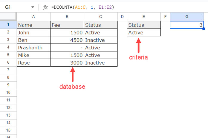
In the following example, we have structured data in the range A1:C as follows:
| Name | Fee | Status |
| John | 1500 | Active |
| Ben | 4500 | Inactive |
| Prashanth | Active | |
| Mike | 1500 | Active |
| Rose | 3000 | Inactive |
Let’s find the following:
- The number of people whose status is “Active.”
- The number of people whose status is “Active” and whose subscription fee is paid.
Steps:
Arrange the criteria in a structured way. Since we need to apply the criteria to the last column (Status), enter the field label of the third column in any empty cell and the criteria below it. For example, enter “Status” in cell E1 and “Active” in cell E2.
Use the following DCOUNTA formula in cell G2 to count the number of active subscribers:
=DCOUNTA(A1:C, 1, E1:E2) // returns 3
Where:
database:A1:Cfield:1(the “Name” column)criteria:E1:E2
Use the following DCOUNT formula to count active subscribers who have paid the subscription fee:
=DCOUNT(A1:C, 2, E1:E2) // returns 2Here, the field is 2, which corresponds to the “Fee” column (a numeric field). The formula counts the numeric values in this column where the criteria in the third column match.
Alternatively, you can use these formulas as well:
=DCOUNTA(A1:C, "Name", E1:E2)
=DCOUNT(A1:C, "Fee", E1:E2)
Hardcoding Criteria in the DCOUNT and DCOUNTA Functions
If you prefer not to use a separate range for entering criteria (like E1:E2), you can use VSTACK, HSTACK, or a combination of both to create an array of criteria. The choice depends on your criteria and may require a detailed tutorial, which you can find in the “Resources” section below.
In the examples provided, you can replace E1:E2 in both the DCOUNT and DCOUNTA functions with the following VSTACK formula:
VSTACK("Status", "Active")Resources
- The Ultimate Guide to Using Criteria in Database Functions in Google Sheets
- Exact Match in Database Functions in Google Sheets – How-To
- How to Use the DSUM Function in Google Sheets
- How to Use the DPRODUCT Function in Google Sheets
- DAVERAGE Function in Google Sheets – Formula Examples
- How to Use the DMAX Function in Google Sheets
- DMIN Function in Google Sheets – How to and Criteria Usage Tips
- Standard Deviation – DSTDEV Database Function in Google Sheets
- DGET Array Formula to Run Down a Column in Google Sheets
- How to Use the DSTDEVP Function in Google Sheets
- How to Use the DVAR Database Function in Google Sheets
- DVARP Function for Conditional Variance in Google Sheets


