In this tutorial, you’ll learn how to count completed tasks in Google Sheets, including cases where tasks have subtasks. While functions like COUNTIF or DCOUNTA might seem sufficient, they only work if there are no task groupings. If you’re dealing with grouped tasks or subtasks, a more dynamic approach is needed.
Let’s explore different formula methods to accurately count completed and incomplete tasks in a project tracking setup.
Simple Case: Single Task Status per Row
If your data uses a single status per row (e.g., “Complete” or a tick box), you can use a basic COUNTIF formula to count:
=COUNTIF(C1:C, "Complete")Or, using a database function:
=DCOUNTA(C1:C, 1, {"Status"; "Complete"})In the DCOUNTA formula, make sure the field label in cell C1 is “Status.” Also, if your data uses tick boxes instead of text, replace "Complete" with TRUE (without quotes).
When COUNTIF Isn’t Enough
The above formulas work well for simple lists, but they fall short when you want to count completed tasks in Google Sheets that are grouped by category (e.g., customer or project), and each group has multiple subtasks.
In that case, we want to count a task as completed only if all of its associated rows are marked “Complete.”
Sample Data and Expected Results
Imagine you’re tracking order statuses for multiple customers:
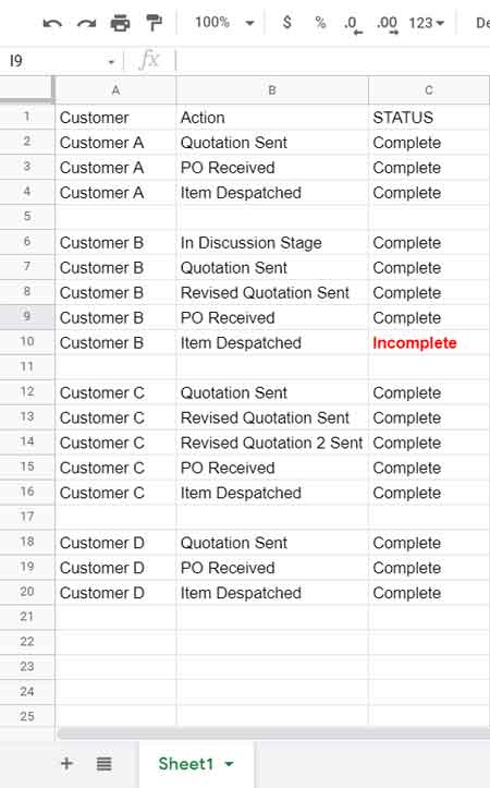
Desired output:
- Completed Tasks: 3 (A, C, D)
- Incomplete Tasks: 1 (B)
Formula to Count Completed Tasks in Google Sheets
Here’s a formula that counts only those tasks (customers) for which all subtasks are marked “Complete”:
=COUNTIF(
  CHOOSECOLS(
     SORTN(
        SORT(A2:C,
          XMATCH(C2:C, VSTACK("Incomplete", "Complete")), TRUE
        ), 9^9, 2, 1, TRUE
     ),3
  ),
  "Complete"
)
Paste this in cell F2. Based on the example above, it will return 3.
Explanation:
A2:C– Your data rangeC2:C– Status columnVSTACK("Incomplete", "Complete")– Sort order: places “Complete” last
This matters because XMATCH uses the position in the array to determine sort order. So, by placing “Complete” last in the VSTACK, we ensure that “Complete” ranks higher, and appears later when sorting — which is essential for SORTN to return the final status per group (which we want to be “Complete” if the group is fully completed)XMATCH(...)– Used for sorting status valuesSORT(...)– Sorts rows based on statusSORTN(...)– Returns the last status for each group (e.g., customer [column #1]), assuming sorted order
| Customer | Action | Status |
| Customer A | Quotation Sent | Complete |
| Customer B | Item Despatched | Incomplete |
| Customer C | Quotation Sent | Complete |
| Customer D | Quotation Sent | Complete |
CHOOSECOLS(..., 3)– Extracts the status column (column #3)COUNTIF(..., "Complete")– Counts fully completed groups
The formula assumes that the last record in each group reflects the group’s overall status, which works if sorted properly.
Formula to Count Incomplete Tasks
Once you know the number of completed tasks, you can calculate the incomplete ones like this:
=COUNTUNIQUE(A2:A) - [Completed Task Count]Just replace [Completed Task Count] with the result from the formula above.
Final Thoughts
Using COUNTIF alone isn’t enough in grouped datasets. By combining SORTN, XMATCH, CHOOSECOLS, and VSTACK, you can dynamically count completed tasks in Google Sheets even when each task has multiple subtasks or rows.
Resources
- Round-Robin Task Assignment in Google Sheets (No Scripts)
- Mark Tasks as Complete When All Subtasks Are Finished in Google Sheets
- Split a Task in Custom Gantt Chart in Google Sheets
- Interactive Random Task Assigner in Google Sheets
- Task Duration, Remaining, and Elapsed Days Calculation in Google Sheets
- Track Remaining Days in Tasks with Sparkline Gantt Charts


Miraculous, Mr. Prashanth. You have a truly miraculous way of mastering and understanding sheets and explaining concepts.
Prasanth you are very knowledgeable.
I have created a sheet.
— link removed by admin —
Essentially my question is how to create column G (detecting the compound word “water world”) and column I (detecting when both the words “water” and “air” are present and outputting evaporation)
I can enter this query in the most relevant sheet.
Hi, Jason,
The Sheet is not editable, but I could view it.
The formula for cell G3 which to be copied down.
=ArrayFormula(LEN(substitute(lower(A3:A12),lower($G$2),"~"))- LEN(SUBSTITUTE(substitute(lower(A3:A12),lower($G$2),"~"),"~","")))The next is an array formula. So first make the range I3:I12 empty, then insert the below formula in I3.
=ArrayFormula(if((gt(C3:C12,0))*(gt(D3:D12,0)),"evaporation","no"))Hello, very valuable advice.
If I have text in A3 is it possible to count compound words with an Array Formula. In this way, it could capture terms such as
"health care"or"Spanish flu".Now it only considers individual terms such as
"health"or"care"=ArrayFormula(countif(transpose(split(A3," ")),"*"&$AH$2:$AV$2&"*"))Hi, Jason,
The question seems not relevant to this article. If you want to look into it, please share an example sheet in the reply.