Are you maintaining your project schedule as well as progress in Google Sheets? Then you may find this tutorial helpful. I have a solution, an array formula, to mark the parent tasks as complete once all of its corresponding subtasks finished.
Let us start with a parent task and its subtasks. Assume you have one task in cell A2, its subtasks in B2:B4 and the status (workflow) of the subtasks in C2:C4.
| A | B | C | |
| 1 | Task | Subtasks | Status |
| 2 | Task 1 | Subtask 1 | Completed |
| 3 | Subtask 2 | Work in progress | |
| 4 | Subtask 3 | Hold |
In a single task that with a few limited numbers of subtasks as above, you can use a logical formula to mark the task as complete.
The following formula in cell D2 will return “Pending” as two of the subtasks are still pending.
=if(and(C2="Completed",C3="Completed",C4="Completed"),"Completed","Pending")Must Read: Combined Use of IF, AND, OR Logical Functions in Google Doc Spreadsheet.
But it won’t work well or become very complex when there are multiple tasks and subtasks in your project schedule. A very tricky use of Vlookup is the most efficient way to mark multiple tasks finished.
Format Data to Mark Tasks as Complete If All the Subtasks Finished
You can use my formula only in structured data as below (A1:C). If your data doesn’t comply with the data in column A to C, you may want to modify your data. See the “Screenshot 2” for unstructured data and how to format that.
Screenshot 1:
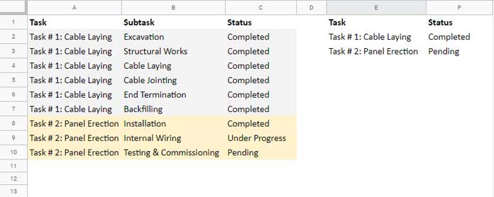
The range E1:F contains my formula and output. Column E contains unique tasks and column F contains whether that tasks are completed or not.
The formula in cell F1 (you will get that below) would mark the tasks as Complete in column F once all the subtasks finished in column C.
See the string “Pending” against task # 2 in cell F3. The reason, it has three subtasks and among them, two tasks are still pending.
Screenshot 2:
I have seen many users using the below format to enter the tasks and subtasks.
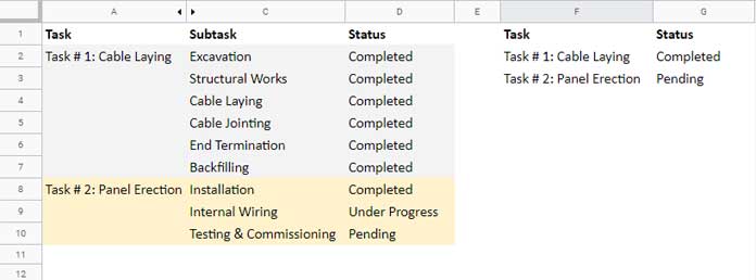
In this case, you can use a helper column to make it structured.
See the “Screenshot 2” again for the hidden column B. In the hidden column B, I have the same data that you can see on the “Screenshot 1” column A. So in the formula I can use B1:D instead of A1:C as the data range.
Here in this example, I am using the data shown on the first screenshot.
Google Sheets Formula to Mark Parent Tasks as Complete
In my example, you can see that the main tasks (parent) are repeated in column A. Using the following UNIQUE formula you can extract the unique tasks in column E.
Formula in Cell E1:
={"Task";unique(A2:A10)}Now we have the unique parent tasks in column E. In cell F1, the following formula marks the completed (parent) task with the string “Completed”.
=iferror({"Status";ArrayFormula(if(vlookup(E2:E,sort({A2:C,if(C2:C="Completed","Z",C2:C)},4,1),4,0)="Z","Completed","Pending"))})The formula checks the subtasks of each parent tasks for completion.
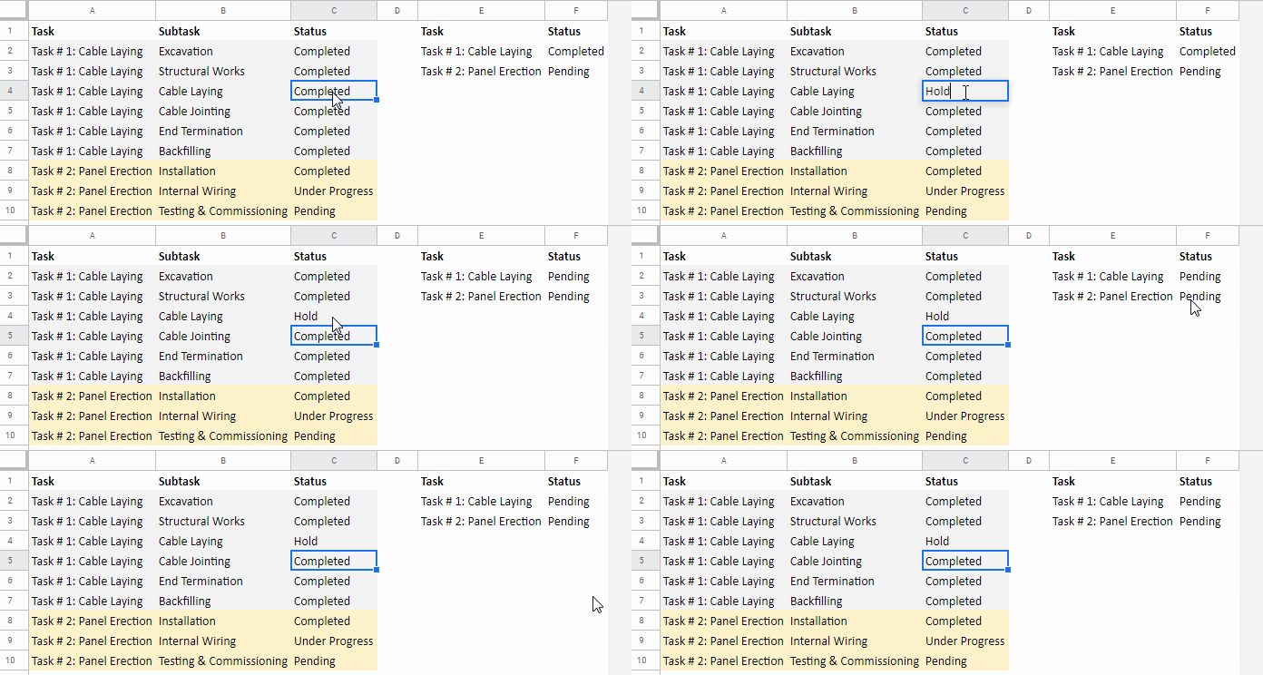
Take the parent task “Task # 1: Cable Laying” for example. It’s in the range A2:A7. All of its subtasks in the range C2:C7 are completed.
When I change one of its subtasks to “Hold” in cell C4, the value in cell F2 is changing from “Completed” to “Pending”.
How the formula marks the tasks as complete once all of its subtasks finished? Here is the formula logic and explanation.
How the Formula Checks Subtasks For Completion
Actually, the core formula used in cell F1 is Vlookup. But you can call it a combination formula as other formulas (SORT and IF) are involved.
Let me explain the formulas used in this combination step by step. I am going to use more screenshots to make you understand the formula clearly.
Step # 1: Moving Completed Subtasks to the Bottom

Actually, the formula underlined in red color is the lookup range in Vlookup. To understand that Lookup ‘range’ first you must know the yellow highlighted IF logical test.
The following is the yellow highlighted formula (except the ArrayFormula) on the above image.
Note: Do not use the ArrayFormula function within SORT.
=ArrayFormula(if(C2:C="Completed","Z",C2:C))Enter this formula in cell D2 to see what it returns. It would return the string “Z” against “Completed” in each row. If the text in column C is not “Completed” then the formula would return that exact text.
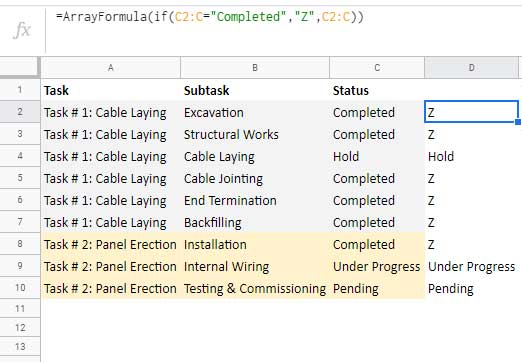
I have added this as the fourth column to the existing data in A1:C using Curly Braces as below.
=ArrayFormula({A2:C,if(C2:C="Completed","Z",C2:C)})Once again see the underlined SORT formula. You can see that I have used the just above formula as the sort range and sorted the fourth column in it in ascending order.
=sort({A2:C,if(C2:C="Completed","Z",C2:C)},4,1)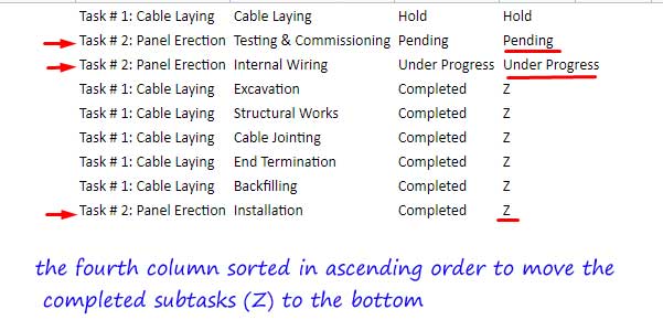
Step # 2: Vlookup to Check Whether All the Subtasks Completed
Why I have sorted the data in ascending order? The Vlookup is the answer to this question.
When sorting the fourth column in ascending order (A-Z), all the completed subtasks, represented by the letter “Z”, will move to the bottom. See the “Task # 2” marked on the screenshot. This sorting has an important role in the Vlookup.
See the Vlookup formula.

Syntax:
VLOOKUP(search_key, range, index, [is_sorted])search_key: The search key in Vlookup is E2:E (two unique tasks).
range: The lookup range is the above sort formula which returns 4 columns. Remember, the fourth column is containing “Z” for finished subtasks and also sorted in ascending order.
index: The index column (output column) is the fourth column that contains “Z” for finished subtasks.
Since there are the same tasks repeated multiple times in the first column in the Vlookup ‘range’, the Vlookup will only return the value from the fourth column of the very first row of the task found.
For example the Task # 2 repeated thrice. Vlookup will return the value “Pending” from the fourth column.
If all of the subtasks are completed, then the Vlookup will definitely return the string “Z”. That means the task is completed. The reason is that we have moved the rows containing “Z” to the bottom. If Vlookup still returns “Z” means, all the subtasks are completed (Z). That’s the logic!
Step # 3: If Formula Tests Vlookup Output for Completion
The outer IF formula tests the Vlookup output. If the value returned by Vlookup is “Z” that means the task is completed.
If the value is any other string, that means there are still pending subtasks under the parent. Accordingly, the formula returns “Completed” or “Pending”.


