Fix the 12th-Month Issue in Google Sheets Formulas

If you use a date column as the criteria column, sometimes you will get incorrect results in conditional count, sum, product, etc., especially when working with the month of December. This post explains how to Fix the 12th-Month Issue in Google Sheets Formulas.

This post is a continuation of one of my earlier posts titled How to Return Blank Instead of 30-12-1899 in Google Sheets Formulas.

Please read that first if you haven’t already because, in that post, I explained the root cause of the 12th-month issue in Google Sheets formulas.

Here’s a quick summary with an example formula.

Quick Background: Why the 12th-Month Issue Happens

I hope you are already familiar with the date functions in Google Sheets. DATEDIF is one of the useful ones. The syntax of this function is:

DATEDIF(start_date, end_date, unit)

Let’s write a simple formula using DATEDIF. First, leave cell C3 blank, and in D4, insert the formula below:

=DATEDIF(TODAY(), C3, "D")

The formula will return #NUM! because the start_date is today’s date and the end_date is blank. In Google Sheets, a blank cell (or a 0 value) is treated as 30/12/1899 by date functions.

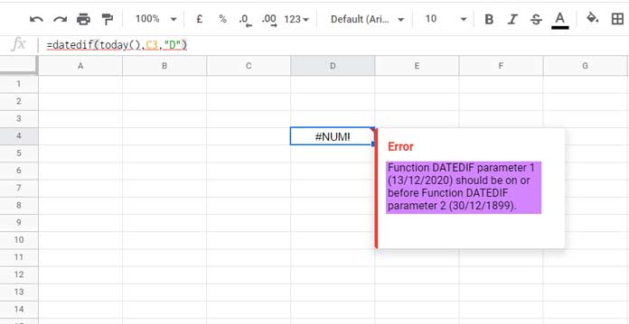
DATEDIF function in an empty cell to demonstrate the 12th-month issue

The reason for the error is simple: the end_date must be greater than or equal to the start_date.

Blank Cell and December Month Error

Since a blank cell is interpreted as 30/12/1899, when you use the MONTH function on a blank cell, it returns 12, which represents December.

Now let’s verify this. Enter the following in any blank cell (other than C3):

=MONTH(C3)

Even if C3 is blank, the formula returns 12. If you type 0 in C3, the result is still 12.

This behavior causes the so-called 12th-month issue in many formulas. Let’s explore how to Fix the 12th-month Issue in Google Sheets Formulas across different scenarios.

How to Fix the 12th-Month Issue in Google Sheets Formulas

I’ll walk you through some basic examples using COUNTIF, SUMIF, QUERY, and SUMPRODUCT. The same principles apply to COUNTIFS, SUMIFS, and a few other functions.

COUNTIF – Wrong Count in December

Here’s a simple COUNTIF formula for the range B2:B15:

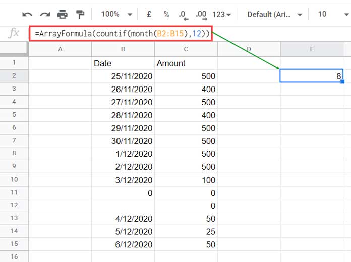
=ARRAYFORMULA(COUNTIF(MONTH(B2:B15), 12))

This formula counts the number of date entries in B2:B15 that fall in December.

Fix the 12th-month issue in the COUNTIF function in Google Sheets

Problem:

If you manually count, you’ll find 6 December dates, but the formula returns 8 because it mistakenly includes the blank (or zero) cells B11 and B12.

Solution:

Filter out blank or zero values:

=ARRAYFORMULA(COUNTIF(MONTH(FILTER(B2:B15, B2:B15>0)), 12))

SUMIF – December Month Issue

Now let’s conditionally sum values in C2:C15 based on December dates in B2:B15.

Here’s the problematic SUMIF formula:

=ARRAYFORMULA(SUMIF(MONTH(B2:B15), 12, C2:C15))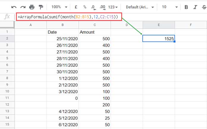

Fix the 12th-month issue in the SUMIF function in Google Sheets

Problem:

The sum returns 1525, which is wrong because it includes values from rows with blank or zero dates (C11 and C12).

Solution:

Use SUMIFS with additional criteria:

=ARRAYFORMULA(SUMIFS(C2:C15, MONTH(B2:B15), 12, B2:B15, ">0"))

Thus, to Fix the 12th-Month Issue in Google Sheets Formulas when using SUMIF, switch to SUMIFS and apply a filter condition.

QUERY – December Month Issue in Query

The QUERY function works a little differently. It uses a month number range of 0 to 11, meaning December is 11.

Here’s a QUERY formula using the same dataset:

=QUERY(B1:C15, "SELECT SUM(Col2) WHERE MONTH(Col1) = 11", 1)

Problem:

The formula incorrectly sums the data and returns 1325 instead of the correct sum.

Reason:

QUERY doesn’t treat blank cells as December, but it does treat 0 as December (month 11). That’s why the sum is different from the wrong SUMIF result.

Solution:

Filter out blank or zero dates:

=QUERY({FILTER(B2:C15, B2:B15>0)}, "SELECT SUM(Col2) WHERE MONTH(Col1) = 11", 1)

SUMPRODUCT – Wrong Product in December

Here’s a basic SUMPRODUCT formula:

=SUMPRODUCT(MONTH(B2:B15)=12, C2:C15)

Problem:

It gives a wrong result by incorrectly considering blanks as December.

Solution:

Again, use FILTER to exclude blank or zero values:

=SUMPRODUCT(MONTH(FILTER(B2:B15, B2:B15>0))=12, FILTER(C2:C15, B2:B15>0))

Wrap Up

To Fix the 12th-Month Issue in Google Sheets Formulas, the trick is simple — use FILTER to exclude blank or zero values before applying your functions.

If you run into any other functions where the 12th-month issue still persists, try applying FILTER first. If that doesn’t fix it, feel free to share your issue with me in the comments — I’d be happy to help!

Thanks for staying till the end. Enjoy!