


Do you know the use of the XMATCH function to find the first or last non-blank cell in Google Sheets? Also, how to highlight them?
You may still be implementing the old-school approaches, like a logical test within MATCH for this.
You may find an example of that approach here: Find the Last Non-Empty Column in a Row in Google Sheets. Of course, that still works.
But if you like to learn new ways to do things in Spreadsheets, you may like this new XMATCH approach.
We will use the wildcard match and reverse lookup feature of this function.
The XMATCH first or last non-empty cell in a row or column type of cell matching has a few advantages.
First and foremost, we can use it to find the range start and range end row or column.
Then there are other things like highlighting those cells and limiting the spill results of ARRAYFORMULA and LAMBDA functions.
For example, if you have values to evaluate in column A, instead of the cell range A1:A, you can specify the following formula as the cell range.
=ARRAYFORMULA(INDIRECT("A1:A"&last_non_blank_cell))So the array formula that uses this range stops spilling at the last non-blank cell. So the cells after that cell won’t return #REF when you enter any value in them.
XMATCH Last Non-Blank Cell in Google Sheets
You may usually scroll horizontally or vertically to find the last non-empty cell in a row or column.
That may usually be time-consuming, with datasets spread across hundreds of rows and columns.
Further, scrolling may not be a solution, if you want to highlight the first or last non-blank cell.
Let me use a small dataset for the example that will help me capture the screenshot of the whole data and explain it.
I have a few product codes in column A. There are also blank cells between a few of the codes. Irrespective of that, I want to match the last code.
Assume we don’t know the value (item code) in the last non-blank cell in column A, which is “ABD113XY”.
If we know, we can use the following formula.
=XMATCH("ABD113XY",A:A,0)How do we XMATCH the last non-blank cell column A when we are unaware of the value in that cell?
Here you go!
XMATCH Last Non-Empty Cell in a Column:
=XMATCH("?*",ARRAYFORMULA(TO_TEXT(A:A)),2,-1)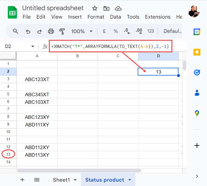
The above XMATCH returns the row number of the last non-empty cell in column A.
Please read the formula explanation below.
Formula Explanation: Wildcard Match and Null Value (Zero Length String)
Syntax: XMATCH(search_key, lookup_range, [match_mode], [search_mode])
We must start with the lookup_range.
I have used the TO_TEXT function with ARRAYFORMULA to convert column A cells to text format. It is a must to perform a wildcard match.
In the process, the said combo converts blank cells to null values (empty strings).
Note:- The null value is the unique string of length 0. So ISBLANK will return FALSE, and LEN will return 0 when testing or evaluating such blank cells.
So the asterisk wildcard isn’t enough to XMATCH the last non-blank cell in column A.
Because, it matches any number of characters, including 0 (null).
But the question mark wildcard matches exactly one character. That justifies the use of ?* as the lookup value.
In the match mode argument, we specified 2, which means we want to perform a wildcard character match, not an exact match.
And the search mode is -1, which means the last value to the first value, i.e., reverse search.
Related: How to Count If Not Blank in Google Sheets [Tips and Tricks].
XMATCH Last Non-Empty Cell in a Row:
Use the same formula after modifying the column range to a row range for this type of value matching in Google Sheets.
The following formula returns the relative position (column number) of the last non-empty string in the first row.
=XMATCH("?*",ARRAYFORMULA(TO_TEXT(1:1)),2,-1)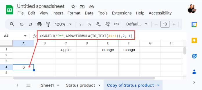
What about the second-row range?
It should be 2:2 instead of 1:1.
Frequently Asked Questions
Q: Should we sort the lookup array in ascending or descending order?
Ans: No. It’s not a requirement.
Q: What about XMATCH’s last non-blank cell position from the nth cell?
Ans: In our examples, we have used A:A or 1:1 as the cell range. It means starting with the very first cell in the sheet. It’s not necessary to stick with that.
If we specify the nth cell, for example, A10:A, you will get the relative position (row number) of the last non-empty cell in this array, whereas A:A will return the row number.
Q: Does this work with numbers, dates, times, and mixed data types?
Ans: Yep! It has no issue with value types.
Q: My last non-empty cell contains an error value. What should I do?
By default, the XMATCH will treat that cell as a blank cell (not a null cell). If you want to consider that error cell as the last non-empty string, use IFERROR as follows.
=XMATCH("?*",ARRAYFORMULA(TO_TEXT(IFERROR(A1:1,"."))),2,-1)XMATCH First Non-Blank Cell in Google Sheets
If you have gone through every bit of information above, you may not find any issue using XMATCH for the first non-blank cell in a row or column in Google Shets.
It’s all about modifying the last argument, i.e., search mode in the formula.
Similar to the XLOOKUP function, XMATCH also has three search modes: 1 (from the first entry to the last entry), -1 (from the last entry to the first entry), 2 (binary search mode when data is sorted in A-Z order), and -2 (binary search mode when data sorted in Z-A order)
In the above XMATCH last non-empty cell, we have used -1 as the search mode. Just replace it with 1.
XMATCH First Non-Empty Cell in a Column:
=XMATCH("?*",ARRAYFORMULA(TO_TEXT(A:A)),2,1)XMATCH First Non-Empty Cell in a Row:
=XMATCH("?*",ARRAYFORMULA(TO_TEXT(1:1)),2,1)Conditional Formatting: XMATCH the First or Last Non-Empty Cells and Highlighting
We can identify the row or column number of the first or last non-empty cell using the XMATCHs above.
How do we use it in conditional formatting, then?
When you want to use XMATCH to highlight the first or last non-blank cell in a row, use the COLUMN function.
Four Highlight Rules
Go to the menu Format > Conditional formatting. Enter A1:Z1 in the “Apply to range” and use the below custom formula.
Formula (Highlighting The First Non-Empty Cell in a Row):
=COLUMN()=XMATCH("?*",ARRAYFORMULA(TO_TEXT(1:1)),2,1)Formula (Highlighting the Last Non-Empty Cell in a Row):
=COLUMN()=XMATCH("?*",ARRAYFORMULA(TO_TEXT(1:1)),2,-1)How do we use XMATCH to highlight the first or last non-blank cell in a column range?
Replace COLUMN with the ROW function. The “Apply to range” is A1:A1000.
Formula (Highlighting The First Non-Empty Cell in a Column):
=ROW()=XMATCH("?*",ARRAYFORMULA(TO_TEXT(A:A)),2,1)Formula (Highlighting the Last Non-Empty Cell in a Column):
=ROW()=XMATCH("?*",ARRAYFORMULA(TO_TEXT(A:A)),2,-1)