


This post explains how to select all or a specific category in multiple columns using the Filter function in Google Sheets.
In Google Sheets, there are three options to perform a filter, one of the most common tasks we do in Spreadsheets.
They are;
- Two menu commands in the DATA menu. They are Create a filter or Filter views > Create new filter view.
- FILTER function.
- QUERY function.
In this tutorial, we are going to learn to use the Filter function to select all or specific category values in multiple columns in Google Sheets.
If you prefer the Data menu, you can easily do it as follows.
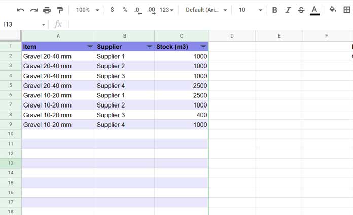
Assume the data is in A1:C, where columns A, B, and C contain Items (text field), Supplier (text field), and Stock (numeric field), respectively.
Steps:
- Select A1:C.
- Click Data > Create a filter.
If you want to filter all the items from “Supplier 1,” click on cell B1 down arrow and uncheck all the values except “Supplier 1.”
- Columns A and C – Set to select all (default).
- Column B – Set to a specific category, i.e., Supplier 1.
If you prefer, you can show the “Stock” equal to or greater than a certain quantity. How?
Click C1 (down arrow) > Filter by condition > Greater than and type 500 in the given field.
To revert to select all in column B, click cell B1 (down arrow) > Select all (link).
How to select all or a specific category in multiple columns using the Filter function in Google Sheets?
Let’s learn that below.
Get Select All in Multiple Columns in Filter Function
Follow the below steps to select all or specific categories in multiple columns in the Filter function in Google Sheets.
There are two main steps and they are the drop-down part and the formula part.
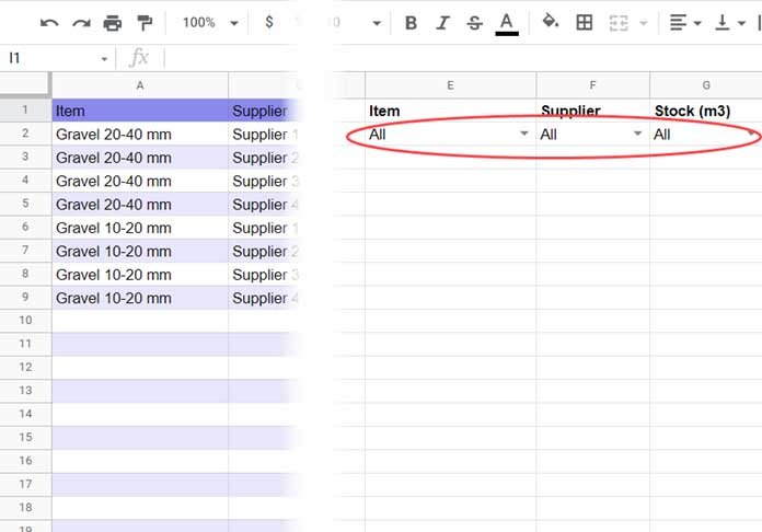
1. Drop-Down Part
As per our sample data, we require to create three drop-down menus for columns A, B, and C and all should contain the option “All” in addition to the unique values from the corresponding column.
We can create them using the Data validation option in Google Sheets. Here is how.
In cell E2 click Data > Data validation and select “List of items” against Criteria. There in the given field, copy-paste the below lists.
Gravel 20-40 mm, Gravel 10-20 mm, AllThey are the unique items from column A and an “All” string. Similarly, create drop-downs in F2 and G2.
List for use in F2;
Supplier 1, Supplier 2, Supplier 3, Supplier 4, AllList for use in G2;
0, 500, 1000, AllNote:- If you prefer to use the “List from a range” against Criteria in the Data validation, then please follow this guide – How to Get an All Selection Option in a Drop-down.
2. Formula Part – Filter Function and Select All in Multiple Columns
In cell E4, insert the following formula.
=filter(A2:C,if(E2="All",row(A2:A),A2:A=E2),if(F2="All",row(B2:B),B2:B=F2),if(G2="All",row(C2:C),C2:C>=G2))How does this formula be able to filter all or selected category values from each column?
For example, we use the following plain Filter formula to filter based on specific conditions in columns A, B, and C.
=filter(A2:C,A2:A=E2,B2:B=F2,C2:C>=G2)To see it working, choose “Gravel 10-20 mm” in E2, “Supplier 2” in F2, and 500 in G2.
You will get the rows matching the above conditions.
The “All” in the drop-downs are not a criterion in columns A, B, and C. But the Filter function will treat it so!
So in our ‘original’ formula, I have used three IF logical tests to make them correctly ‘readable’ to the Filter function.
For example, the highlighted part in if(E2="All",row(A2:A),A2:A=E2) tests whether the E2 value is “All” or not.
If it’s “All,” the filter criterion in column A is row(A2:A), and if not, A2:A=E2.
You may doubt whether row(A2:A) is a condition in Filter.
Yep! It defines a condition similar to len(A2:A). The difference is as follows.
row(A2:A) – It means have row numbers.
len(A2:A) – It means whether the rows have values or not.
I prefer the former to get select all in columns in Filter.
If you want select all but exclude blank cells in that column, use the latter.
That’s all. Thanks for the stay. Enjoy!
Resources
- How to Apply Unique in Selected Columns in Google Sheets.
- How to Randomly Select N Numbers from a Column in Google Sheets.
- Dynamic Formula to Select Every nth Column in Query in Google Sheets.
- Select Only the Required Column from an Array Result in Google Sheets.
- A Drop-down Menu in Google Sheets to View Content from Any Sheets.
- Auto-Populate Information Based on Dropdown Selection in Google Sheets.
- Distinct Values in Drop Down List in Google Sheets.
- Create a Drop-Down to Filter Data From Rows and Columns.
- Create a Drop-Down Menu From Multiple Ranges in Google Sheets.
- How to Combine Multiple Sheets in Importrange and Control Via Drop-Down.