


You should learn all possible data manipulation techniques as they can come in handy at any time in the future. Learn new tips for working with Google Docs Spreadsheets. With the SUMIF function, you can sum every nth row or column in Google Sheets.
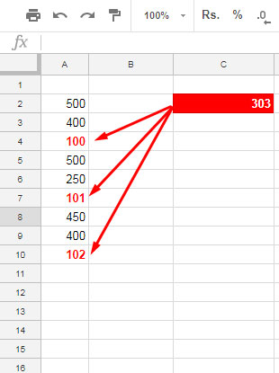
The nth row can be every third, fourth, or fifth row, or a repetition of any specific row number.
For example, let’s sum every third row. But don’t worry, you can easily customize this formula to sum any nth occurrence.
As mentioned above, for this purpose, I am using the popular SUMIF function.
The Formula to Sum Every Nth Row in Google Sheets
Here is the formula to sum every 3rd row in the range A2:A in Google Sheets:
=SUMIF(ARRAYFORMULA(MOD(SEQUENCE(ROWS(A2:A)), 3)), 0, A2:A)You can easily tweak this formula to sum every custom number of rows, such as every 4th, 5th, or 6th, or a repetition of any nth rows.
For example, if you want to sum every 5th row, please change the number 3 to 5 in the formula.
Formula Explanation
First, let’s understand the formula arguments. That’s the easiest way to learn a formula.
The SUMIF Syntax:
=SUMIF(range, criterion, [sum_range])Where:
range:ARRAYFORMULA(MOD(SEQUENCE(ROWS(A2:A)), 3))criterion: 0sum_range: A2:A
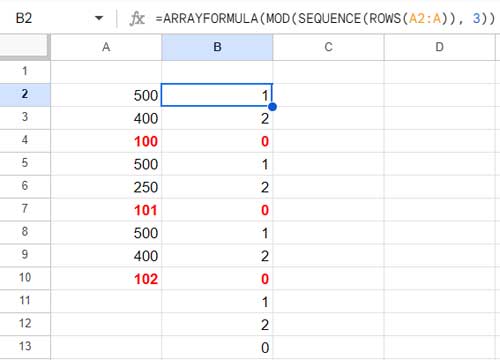
The range in this SUMIF formula is the most important part of it. It returns 0 in every 3rd row starting from row #2.
The SUMIF sums the sum_range A2:A if the range is equal to 0. Now, let’s delve into the ‘range’ part of the formula in detail.
Actually, a MOD formula acts as the range in SUMIF. So, I should explain the use of the MOD formula.
The MOD function Syntax:
=MOD(dividend, divisor)The MOD function returns the remainder after a division operation.
Consider this formula used as the range in the above SUMIF formula:
=ARRAYFORMULA(MOD(SEQUENCE(ROWS(A2:A)), 3))Where:
dividend:SEQUENCE(ROWS(A2:A))
The SEQUENCE function returns sequence numbers from 1 to n, where n is represented by ROWS(A2:A), i.e., the number of rows in the range.
divisor: 3
The MOD function takes these serial numbers as the dividend and 3 as the divisor.
Note: We include the ARRAYFORMULA function because MOD is a non-array function and we’re feeding an array into it.
The MOD formula returns the value 0 in every third row since the divisor is 3. If you use 5 as the divisor, then the formula will return 0 in every fifth row.
In SUMIF, I’ve set the criterion as 0. So, the SUMIF formula will only sum the rows where the value in the range (you can say virtual MOD formula range) is 0.
That’s all. This way you can sum every nth row in Google Sheets.
Summing Every Nth Column in Google Sheets
You can sum or add every nth column in Google Sheets as detailed above, similar to adding nth rows.
How?
You need to make two changes in the formula:
In the above formula, you should replace the ROWS function with the COLUMNS function because we want to find the number of columns in the range, not rows.
In the formula that sums every nth row, we use the SEQUENCE function to return numbers vertically in the syntax SEQUENCE(rows). What we want here is sequence numbers horizontally in the syntax SEQUENCE(rows, columns) where rows should be 1 and columns should be COLUMNS(range).
To sum every third column in the range E2:Z2, you can use the following formula:
=SUMIF(ARRAYFORMULA(MOD(SEQUENCE(1, COLUMNS(E2:Z2)), 3)), 0, E2:Z2)The n here is 3. Replace that number with 10 to sum every 10th column.
Resources
Here are some related resources for Google Sheets.
- Vlookup to Find Nth Occurrence in Google Sheets [Dynamic Lookup]
- How to Highlight Every Nth Row or Column in Google Sheets
- How to Copy Every Nth Cell in a Column in Google Sheets
- Dynamic Formula to Select Every nth Column in Query in Google Sheets
- Delete Every Nth Row in Google Sheets Using Filters
- Extract Every Nth Line from Multi-Line Cells in Google Sheets
- Import Every Nth Row in Google Sheets Using Query or Filter (Same File)
- Highlight Nth Occurrence of a Value in Google Sheets
- XLOOKUP Nth Match Value in Google Sheets
- INDEX MATCH Every Nth Column in Google Sheets
Hi Prashanth,
I have a similar question: how can I sum within an interval of x cells?
Example:
Dragging =sum(A1:A6) gives me =sum(A2:A7). I’d like to have a way to drag and obtain =sum(A7:A13)
I have a set of daily data that I need to sum up weekly.
Thanks in advance.
Hi, Homelader,
I don’t know how many weeks of data you have.
For example, I assume you have 12 weeks of data.
In cell C1, insert the following Sequence formula. It will return the multiplications of 7 in C1:C12.
=sequence(12,1,1,7)In D1, you may insert the following formula and copy-paste it down.
=sum(chooserows($A$1:$A,sequence(7,1,C1)))I’ll try to make it an array formula that runs without helper cells in the near future. I’ll try to share that tutorial with you then here.
Hello Prashanth
I think this article is what comes closest to what I want to achieve. However, I can’t seem to make it work with what I got.
I want to sum every other row in an area if the text below it matches my reference.
Hi, Alexander Kolby,
For this question, an example sheet would be easy for me to understand the data you want to process. You can leave the URL in the comment (I won’t make it public).
Hi Prashanth,
Is it possible to SUMIF excluding every nth row? What would the formula look like?
-Angela
Hi, Angela,
We can use SUMIFS.
We can use the following formula if sum_range is B3:B and criteria_range1 is A2:A.
=ArrayFormula(sumifs(B3:B,A3:A,"Apple",mod((row(A3:A)-row(A3)+1),16),">1"))
Replace “Apple” with your criterion. The formula excludes every 16th and 17th row.
Just for every 16th row, replace
>1with>0.Hey, I was wondering whether you can tell me how to sum x number of rows repeatedly where x can be variable?
For example, let’s say I have a row with numbers 1,2,5,4,2,8,5,7,8,4,9,6,3.
If I want to sum three numbers, I can put the sum formula against 5 with the cell range A1 to A3.
Then drag the ‘+’ to get the sum for A2:A4, A3:A5, etc.
However, I want to read the range length three from a different cell.
How would I do that? Thanks.
Hi, Cvan,
Assume the values to sum are in A1:A and the variable (x) that determines the sum range is D2.
Enter 3 in D2. Now instead of
=sum(A1:A3), you can try=SUM(offset(A1,0,0,$D$2)).If the D2 value is 4, the above SUM and OFFSET combo will return the value that is equal to
=sum(A1:A4).Hi Prashanth,
Thank you for the great explanation!
I’m having trouble adapting the formula to achieve the following: I want to sum in every column (from A:E) only the values in the row “5M”… how could this be achieved?
# | A | B | C | D | E
EP | 1 | 3 | 5 | 6 | 3
5M | 3 | 5 | 6 | 8 | 8
Ko | 4 | 3 | 7 | 9 | 1
EP | 4 | 4 | 5 | 6 | 7
5M | 1 | 8 | 6 | 2 | 6
Ko | 1 | 3 | 5 | 6 | 3
EP | 3 | 5 | 6 | 8 | 8
5M | 4 | 3 | 7 | 9 | 1
Ko | 4 | 4 | 5 | 6 | 7
Thank you for a short reply.
Best regards
Dan
Hi, Dan,
When I enter your data in my Sheet, it occupies the range A1:F10.
First, make B11:F11 empty. Then in cell B11, use the below Query or DSUM.
QUERY:
=query(A1:F10,"Select Sum(B),Sum(C),Sum(D),Sum(E),Sum(F) where A='5M' label Sum(B)'',Sum(C)'',Sum(D)'',Sum(E)'',Sum(F)''",1)DSUM:
=ArrayFormula(dsum(A1:F11,B1:F1,{"#";"5M"}))When you use this formula, please make sure to change the “#” inside the formula with the actual value (field label) in cell A1. Because database functions are very sensitive to field labels.
Thank you very much! Good solutions!
Meanwhile, I also found one solution:
=sum(FILTER(B1:F11;mod(row(B1:F11);3)=0))whereas, the “3” ist the n-th row you want to sum up.
Have a great day!
Dan
I wish you could have an example for columns that are as detailed as this example is for rows.
Hi, Kari,
Thanks for your feedback.
Hey,
I’m pasting this formula:
=sumif(ArrayFormula(mod((row(A12:A)-row(A12)+1);3));0;A12:A)I use
;instead of,because of my Spreadsheet settings. But I’m getting an alert message that says: “Error Reference does not exist.”Do you know why could be?
Hi, Mairus,
The formula seems perfect to me. It did work in my test.
You can use this formula in any column other than column A to sum every 3rd occurrences. It will possibly sum the values in cell A14, A17, A20…
If possible, replicate the error in a demo sheet and share it with me. So that I can find out the cause.
You can read this tutorial to know some of the errors in Sheets and reasons – Different Error Types in Google Sheets and How to Correct It.
Best,
Hi Prashanth,
Is it possible to average every nth column, similar to the image you showed in the Additional Tips section?
Note: The provided link has been removed by the admin.
For example, in cell B3 I’d like to average all of the Data 1 columns in each row (so E3, I3, M3,, Q3, etc…), and do the same for C3 with Data 2 and D3 with Data 3
Hi, Gabe,
Use the below formulas and copy (drag) down.
Cell B3:
=averageif(ArrayFormula(mod((column($E$1:$T$1)-COLUMN($E$1)+1),4)),1,E3:T3)Cell C3:
=averageif(ArrayFormula(mod((column($E$1:$T$1)-COLUMN($E$1)+1),4)),2,E3:T3)Cell D3:
=averageif(ArrayFormula(mod((column($E$1:$T$1)-COLUMN($E$1)+1),4)),3,E3:T3)I may write a detailed tutorial on this and link you back later.
Best,
Hi, I tried to edit your formula but I keep getting an error. Here is an example of my table.
“https://docs.google.com/spreadsheets/d/1XdJd9BP8QIy_anLeroIFZCriLwUcxM0EjiJsc5E0Wb0/edit?usp=sharing”
I would like to sum Data5, every 10th row. Could you help me?
Hi, Sudinea,
Please note that as per your Google Sheets File > Spreadsheet settings, you must use a semi-colon instead of a comma in your formulas.
How to Change a Non-Regional Google Sheets Formula.
So the formula would be as follows.
=sumif(ArrayFormula(mod((row(A6:A)-row(A6)+1);10));0;B1:B)But this simple SUMIF formula would also work.
=sumif(A6:B64;"Data5";B6:B64)Sum every nth row but the first row is not the nth row.
Example:
If you want to sum every 10th rows but starting from the 11nth row, then tweak the formula as below.
=sumif(ArrayFormula(mod((row(A6:A)-row(A6)+1);10));0;B2:B)Best,