It’s always a better idea to keep the numbers simple or we can say clean by rounding them. So here comes the importance of the ROUND functions in Google Sheets.

There are certain rules regarding rounding numbers. The Round functions in Google Sheets are no exception to this.

Here in this post, you can quickly learn how to use Google Sheets three commonly using round functions and how they round numbers. The functions are ROUND(), ROUNDUP(), AND ROUNDDOWN().

Let’s start with the ROUND() function. Learning this function is a must to easily grasp the other two siblings of this function.

ROUND Function in Google Sheets

The purpose of the ROUND() function in Google Sheets is to round a number to a certain number of decimal places as per standard rules.

Syntax:

ROUND(value, places)

Arguments:

value – The value that you want to round.

places – The number of digits (decimal places) to which to round the value. It’s optional and the default value is 0 digit (decimal place).

The below examples will give you an idea about the said standard rules in rounding numbers.

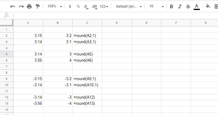
There are 8 numbers (values) to round in cell range A2:A13 and the first number to round is 3.15 in cell A2. The number of ‘places’ to round is 1 in the ROUND formula in cell B2.

The formula rounds the number to 3.2 because as per the standard rule the digit to the right (the next most significant digit) is considered which is 5 in 3.15 here.

As per the standard rule, if the next most significant digit is;

>=5 – the digit is rounded up.
<5 – the digit is rounded down.

Please see the value in cell A3 which is 3.14. In this, the next most significant digit is 4. So the formula =round(A3,1) rounds down the digit and the result is 3.1.

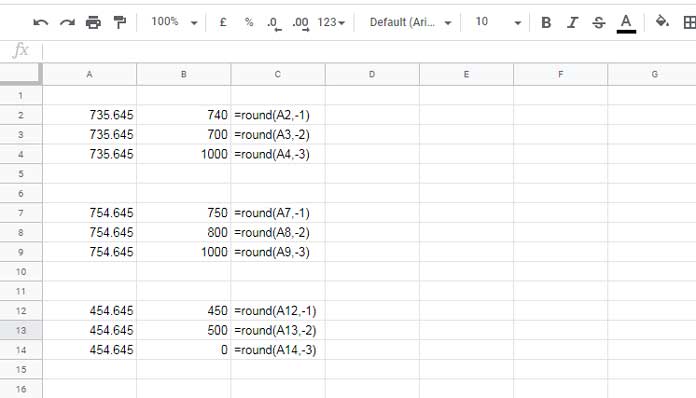
The ‘places’ can be negative in the ROUND function in Google Sheets. In that case, the value is rounded to the left of the decimal point.

Please go through the below formulas and results to master the negative places use in the ROUND function in Google Sheets.

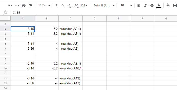
ROUNDUP Function in Google Sheets

The purpose of the ROUNDUP() function is to always round up a number to a given number of decimal places. It behaves/operates like ROUND() except the fact that it always rounds up a number.

Syntax:

ROUNDUP(value,[places])

Arguments:

value – The value that you want to round up.

places – The number of digits (decimal places) to which to round up the value (an optional argument and the default value is 0).

Example Formulas

+ve Places in the ROUNDUP Function in Google Sheets:

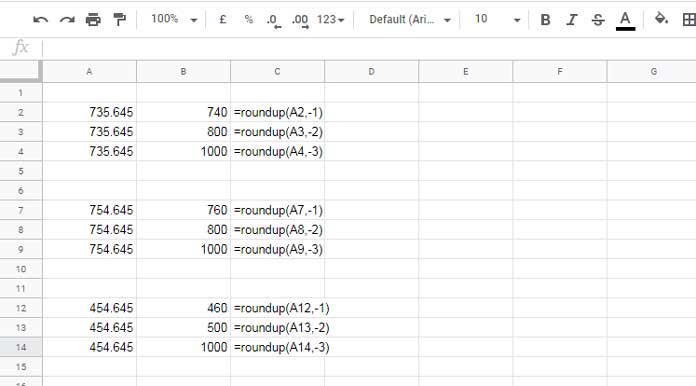
-ve Places in the ROUNDUP Function in Google Sheets:

ROUNDDOWN Function in Google Sheets

The purpose of the ROUNDDOWN() function is to always round down a number, toward 0. This function also behaves/operates like ROUND() except the fact that it always rounds down a number.

Syntax:

ROUNDDOWN(value,[places])

Arguments:

value – The value that you want to round down.

places – The number of digits (decimal places) to which to round down the value. It’s an optional argument and the default value is 0.

Example Formulas

+ve Places in the ROUNDDOWN Function in Google Sheets:

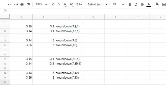
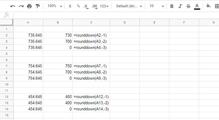
-ve Places in the ROUNDDOWN Function in Google Sheets:

Combined Use with Other Formulas

The above are examples of how to use the Round Functions in Google Sheets.

You can use the above functions in combination with functions like SUM, DSUM, SUMPRODUCT, SUMIF, etc. by just wrapping the corresponding formulas. See a few examples below (excluded explanations).

ROUND Function with SUMIF:

=round(sumif(B5:E9,B13,C5:C9),0)

Similarly, you can use ROUNDUP as well as ROUNDDOWN functions with the SUMIF function.

ROUNDDOWN function with DSUM:

=rounddown(dsum(B6:D14,3,B2:D4),1)

ROUNDUP function with SUMPRODUCT:

=roundup(sumproduct((B7:B14="Myron Ambriz")*((C7:C14="North")+(C7:C14="South"))*(D7:D14)),0)

Conclusion

When we use Google Sheets to create invoices or anything related to money, it is better to limit the number of decimal places to two or zero.

You can use any of the Round functions above in such cases. A simple number is always easy to remember, right?

There are a few more Round functions in Google Sheets like TRUNC, MROUND, etc. I think it’s better to write a separate post for that.

Similar:

• How to Use Google Sheets TRUNC Function.
• How to Use the MROUND Function in Google Sheets.
• Round, Round-Up, Round-Down Hour, Minute, Second in Google Sheets.
• How to Use the Floor Function in Google Sheets.
• How to Use the Ceiling Function in Google Sheets.
• Round Numbers in Google Sheets Query – Workaround.
• How to Round Percentage Values in Google Sheets.