There are no built-in functions to find the cell address of a last used cell in Google Sheets. But I’ve two custom formulas to do this.

Keep one thing in mind if you opt to use any of them. Both of the formulas may fall short of returning a perfect result if there is any blank cell in the ‘primary’ column in the range. I’ll explain it.

Primary Column:

In your data range, there may be multiple columns. For example, a range like A1: G has 7 columns and infinitive rows.

In this, you can set any column as primary in my formula. For example, you can use Column A.

The formula may revolve around this column and blank cells in this column can return wrong results. So choose a column that does not contain blank cells in your range.

This formula is different from what you may think!

Normally with a lookup formula, we can find the cell address of a lookup value. But here the case is different. We are here to find the cell address of a last used cell, not the cell address of a search key found.

How to Find the Cell Address of a Last Used Cell in Google Sheets

Formula 1:

I’ve used three functions here to find the cell address of a last used cell in a range. The functions are CELL, INDEX, and COUNTA. But the main function in this formula is, of course, the INDEX.

Formula Explanation:

First, let me explain the role of Index function here.

With the Index function, my aim is to return the last cell value. From this value, we can find the last cell address.

Syntax:

INDEX(reference, [row], [column])

Formula:

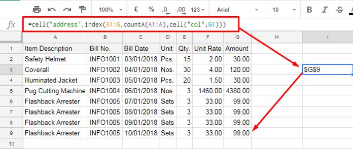
=INDEX(A1:G,countA(A1:A),cell("col",G1))

Here we have already the “reference” to use in Index and it’s A1: G. Now we want to find the last row number in our data range.

Here I’ve used CountA function in Column A which is my primary column here. Of course, CountA has an edge over the Count function as it accepts both numbers as well as text in the count.

It’s easy to find the column number as we know our last column in the data range is column G.

You can directly put 7 as G represents column number 7. Alternatively, the Cell formula returns Column number of G. Actually here the formula is like;

=INDEX(A1:G,9,7)

Result: 99 (the last cell value in the range in G9.

You can use the above Index formula to return the last cell value in a range. Remember! not last used cell address.

Now we can use the Cell function “address” info type to return the address of this cell containing the value 99.

Formula

=CELL("ADDRESS",index(A1:G,9,7))

Which is equal to

=CELL("address",index(A1:G,countA(A1:A),cell("col",G1)))

Result: $G$9

Formula 2

Here is one more formula to find the Cell Address of a last used cell in Google Sheets. This’s an entirely different approach.

As you can see the main functions here in this example are ADDRESS, ARRAYFORMULA, MIN, IF and ROW.

The below formula is the main part here and here my primary column is G. So any blank cell in this column possibly return a wrong result.

=ArrayFormula(MIN(IF(G2:G="",ROW(G2:G)-ROW(G2)+1)))

Result: 9

Formula Explanation:

When you use this formula independently, after removing the MIN, for example in H2, it may return serial number 1,2,3 starting from H2 to downwards.

But the IF logical function may force the formula to put serial number only in H10. Because the formula only returns numbers wherever the cell value in G is blank.

That means it only returns the number 9 in H10 as G10 is blank and in all the other cells, it returns FALSE. The MIN function in this range returns the number 9.

If you have still doubt, I have a detailed tutorial on this. Please check that.

Similar: How to Count Until a Blank Row in Google Sheets

So the formula is;

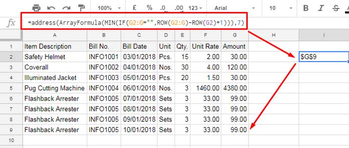
=address(ArrayFormula(MIN(IF(G2:G="",ROW(G2:G)-ROW(G2)+1))),7)

Which is equal to;

=address(9,7)

Result: $G$9

That’s all. This way you can find the Cell Address of a Last Used Cell in Google Sheets.