How to Count Until a Blank Row in Google Sheets

Sometimes you may need to count until a blank row from the beginning of a table. This can be accomplished using XMATCH in Google Sheets.

For example, you have dates in column A and “x” marks in column B. An “x” mark indicates that a delivery has been made on the corresponding date in column A.

In this case, you can count from the first cell to the blank cell in column B to determine the number of days without an uninterrupted supply.

You can follow the same approach if you want to count until the first entirely blank row in a range; the formula will require some minor adjustments.

Table of Contents

Count Until the First Blank Cell in a Column

The following formula returns the count of values in B2:B until the first blank cell:

=ArrayFormula(XMATCH(TRUE, B2:B="")-1)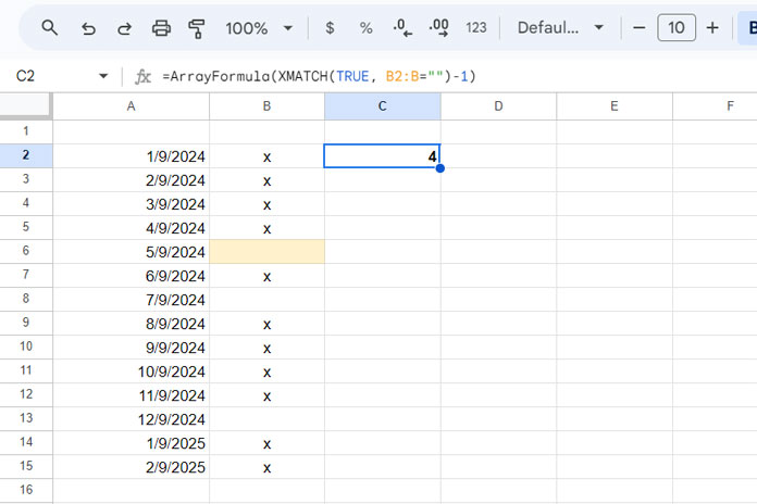

Count Until the First Blank Cell in a Column

The XMATCH function finds the first occurrence of TRUE in an array of TRUE or FALSE values, where TRUE represents empty cells and FALSE represents non-empty cells. The logical expression B2:B="" checks whether each cell is blank or not.

The formula returns the relative position of the first empty cell. To get the count of values up to that empty cell, we subtract 1 from the result.

We use ARRAYFORMULA because the logical expression operates over an array of cells.

Count Until the First Blank Row in a Range

Sometimes, you may leave an empty row to separate sections.

For example, let’s say we have dates, purchase order quantity, and delivery status in the range A1:C.

Each blank row between the data represents a new day. How do you count up to the first blank row in the range A2:C, excluding the header row?

We can use a similar formula to the one we used earlier, but with a combined range in the logical expression:

=ArrayFormula(XMATCH(TRUE, A2:A&B2:B&C2:C="")-1)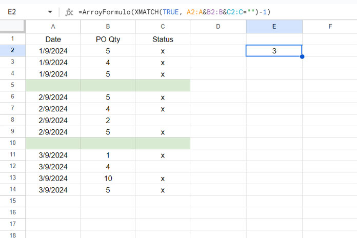

Count Until the First Blank Row in the Range

Here, the logical expression A2:A&B2:B&C2:C="" combines values from columns A to C row by row and checks whether the combined output is blank.

The formula elements are the same as in the earlier example.

Additional Tips

You can replace XMATCH with MATCH as well. However, simply replacing XMATCH with MATCH is not enough.

In the above example, we followed the XMATCH syntax: XMATCH(search_key, lookup_range), where the search_key is TRUE, and the lookup_range is the logical expression.

When using MATCH to count until the first blank cell in a column or range, you must specify 0 as the third argument to indicate that the data is not sorted.

Syntax: MATCH(search_key, range, search_type)

Resources

Here are some related resources for further exploration: