


I have a sales report in Google Sheets where I want to extract only the top 5 items based on sales volume. Is it possible, and if possible, how to do that? Yup! It’s possible in Google Sheets. Let’s see how to extract the top N number of items from a list in Google Sheets.
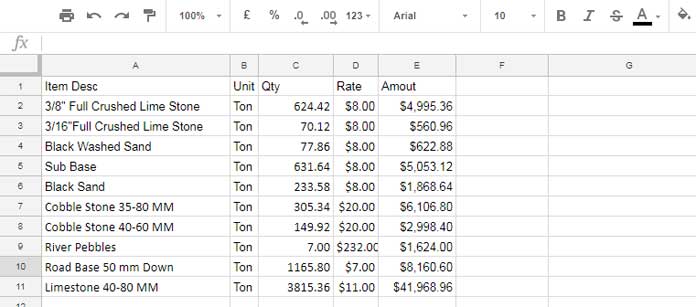
My below sample sales report contains sales volume, unit rate and sales amount of some landscaping materials.
From this list, I want to extract the top 5 items based on the volume of sales. You can see the sales volume of each item in column C in tonnage.
How to Extract Top N Number of Items from a Data Range in Google Sheets
Here, I’ve only a small amount of data in the sales report. I set it so to enable you to manually match the formula output with the tope N numbers in the dataset.
Here I’m going to extract the top 5 number of items from this data range by using Google Sheets Query Function.
Formula and Result:
=Query(A1:E,"Select A,B,C,D,E where A<>'' Order by C Desc Limit 5")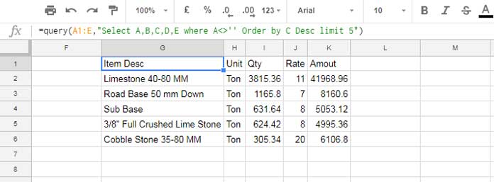
The above Query formula can return the result that we want.
If you know the usage of Query formula in Google Sheets, you can easily change the number of items to be returned.
For that, you just want to change the number used in the Limit clause. I mean you can change the “limit 5” to “limit 3” to return the top 3 items.
You May Also Like: What is the Correct Clause Order in Google Sheets Query?
If you are not familiar with the Query, I can explain to you how this formula works.
Formula Explanation
The above formula sorts column C by descending order. So what happens?
It would return the items based on their sales volume as I have the sales volume in Column C.
In the Query formula, I’ve used the “limit” clause to restrict the returned rows to 5. As a result, the formula returns top 5 items based on their sales volume in Column C.
You can change the limit clause row number to 10 to extract the top 10 number of items.
To use this formula with your own data, you may only want to change the data range in the formula like A1:E to your data range.
If your data range is spread across A1:D, then the columns in “Select” clause must be like “Select A,B,C,D” or “Select *”.
This’s the possibly one of the easiest method to extract the top N number of items from a data range in Google Sheets.
As a side note, you can also get the same result by using Filter, Sortn (sorted N rows) or some other formulas in Google Sheets.
Here is the SORTN alternative to Query to extract the top 5 rows. The # 5 in the below formula represents the ‘N’.
=sortn(A2:E,5,0,3,0)This formula has a feature. If you change the # 0 to 1 in the formula, then it would return the top 5 rows + 1 additional row identical to the fifth row, if any.
Thanks so much!
Is there a way to add a condition to it?
So, for your example, if you had another column titled “product type,” and you wanted the top quantity sales for all sand products?
Hi, Abigail Ryan,
Assume column F contains the “Product Type.”
Here are the formulas based on it.
Query:
=Query(A1:F,"Select A,B,C,D,E where lower(F)='sand' Order by C Desc Limit 5")SORTN:
=sortn(filter(A2:E,F2:F="Sand"),5,0,3,0)Possible to set the limit to be dynamic to a cell reference?
Hi, Brad,
We can do that. In the below example, cell E1 controls the Query Limit clause.
=Query(A1:B,"Select A,sum(B) group by A order by sum(B) desc limit "&E1&" label sum(B)'Sales'")This was great. Exactly what I was looking for.
You saved me a ton of time, thanks!
You should leave the formula in the article.
Hi, Brendan,
Sorry for the inconvenience. I’ll update the post by today itself.