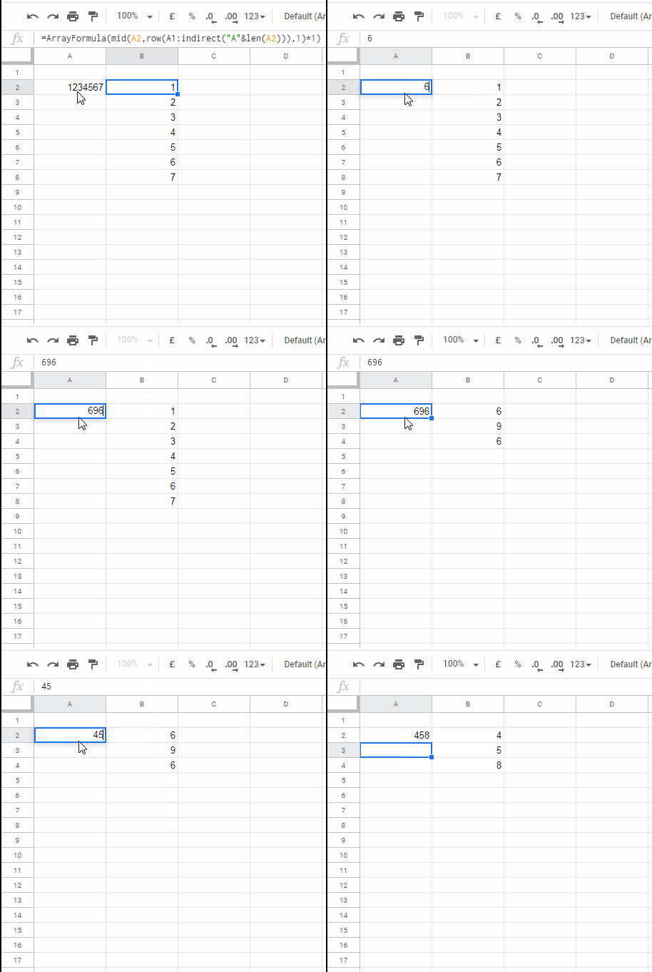
You can effortlessly split a number into its individual digits in Google Sheets using the MID function as an array formula. This tutorial is dedicated to teaching you how to utilize the MID ‘text’ function for this purpose.

While MID is primarily a text function, it can be used to effectively separate numbers into individual digits.

In this tutorial, you will learn two key aspects: a useful technique for splitting numbers into digits and the proper utilization of the MID function in Google Sheets.

I will guide you through the steps to split a number into its individual digits, which means separating them into separate cells within Google Sheets. But before we dive into that, let me introduce you to the syntax and arguments of the MID function in Google Sheets.

Syntax of the MID Function

Syntax:

MID(string, starting_at, extract_length)

Arguments:

• string: The text from which to extract a substring.
• starting_at: The index from the left of the text, indicates where to begin extraction. The first character in the text is at index 1.
• extract_length: The length of the substring to extract. If the extract_length exceeds the available length, the function will return the remaining characters in the string, starting from the starting position.

Before we start how to split a number into digits, let’s look at a MID function example below.

MID Formula Example:

=MID("InfoInspired",5,8)

The above MID formula will result in “Inspired.”

As per the syntax, “InfoInspired” is the string. Using the formula above, we have extracted 8 characters (the extract_length) starting from the character at the 5th position (the starting_at), which is “I.” Therefore, the result is “Inspired.”

This functionality allows us to extract any number of characters from any position within a given string. It is also applicable to numbers, as the MID function treats numbers as strings.

This answers questions about how to extract or separate a part of a word or sentence in Google Sheets. However, it’s worth noting that there is an even more powerful function called REGEXEXTRACT.

How to Split a Number into Digits in Google Sheets Using the MID function

As previously mentioned, MID in Google Sheets is a text function that treats numbers as strings. You can utilize the same method described above to split numbers.

Here’s an example of how to use MID with numbers to split a number into its individual digits in Google Sheets.

This is a non-array formula, which means we will use individual functions for each digit. Afterward, we’ll explore how to separate each digit all at once.

Example

In cell A2, type the number 1234567, which we are going to split into individual numbers.

In cell B2, insert the following formula:

=MID(A2, 1,1 ) * 1

This will return the first digit. In C2, insert the same formula, then replace starting_at 1 with 2.

=MID(A2, 2, 1) * 1

In each subsequent step, replace starting_at with the next number in the sequence.

Since there are 7 digits in the number in cell A2, observe how I’ve extracted each number using 7 MID formulas in cells B2 to H2. Another example is included in the 3rd row.

Note: We can use the MID text function to split numbers and obtain the result (digits) in numeric format by multiplying the result by 1.

Dynamic MID Formula in Google Sheets (MID Array Formula)

Rather than using multiple MID formulas, you can automate the extraction process with the help of the ROW or SEQUENCE function, as shown below.

We will split a number into digits, but you can follow the same approach to separate characters in a string. To do this, simply remove *1 from the formula.

MID with ROW to Split Numbers into Digits

Take a look at this formula:

=ARRAYFORMULA(MID(A2, ROW(A1:A7), 1) *1)

The ROW function provides the numbers 1 to 7 to the starting_at argument of the MID function.

The formula above extracts the numbers 1 to 7 (assuming the number in cell A2 is 1234567) and displays them vertically.

If you prefer the result to be displayed horizontally, simply wrap the formula with TRANSPOSE.

=ARRAYFORMULA(TRANSPOSE(MID(A2, ROW(A1:A7), 1) * 1))

However, the formula above is not dynamic. It currently assumes there are 7 digits in the number in cell A2, which is why we use A1:A7 in the ROW function. If there are 11 digits, you’d need to adjust the row formula range to A1:A11.

The following formula addresses this issue. It can split any number into separate cells, regardless of the number of digits. This formula utilizes the INDIRECT and LEN functions for this purpose.

=ARRAYFORMULA(MID(A2, ROW(A1:INDIRECT("A" & LEN(A2))), 1) * 1)

MID with SEQUENCE to Split Numbers into Digits

I’m replacing the previous formula in cell B2 with this MID, SEQUENCE, and LEN combination. It’s another array formula for splitting a number into digits in Google Sheets.

=ARRAYFORMULA(MID(A2, SEQUENCE(LEN(A2)), 1) * 1)

Here, the SEQUENCE(LEN(A2)) provides the numbers 1, 2, 3, and so on up to the length of the number in A2 for the MID function.

This is a dynamic array formula.

Conclusion

I hope you have grasped the steps to split numbers into digits in Google Sheets.

Now, you might be wondering, why should someone split or separate digits within a number.

I have utilized this function in creating a number-to-word converter in Google Sheets. We can’t anticipate how users might apply a function dynamically in their spreadsheets, so the possibilities are entirely up to the users.

Resources:

1. How to Split Number from Text When No Delimiter Present in Google Sheets.
2. Extract First, Last, and Middle Names in Google Sheets.
3. How to Match | Extract Nth Word in a Line in Google Sheets.
4. Extract All Numbers from the Text and SUM It in Google Sheets.
5. Split to Column and Categorize – Google Sheets Formula.
6. Split a Column into Multiple N Columns in Google Sheets.
7. Extract Vowels and Consonants Separately in Google Sheets.
8. Extract Unique Values from a Comma Separated List in Google Sheets.
9. Formula to Reverse Text and Numbers in Google Sheets.