A few days ago, one of my readers requested a formula to return all the working dates between two dates in Google Sheets.
They specifically wanted to exclude weekends and list all the working dates between a start date and an end date.
I took it one step further! In addition to generating a list of dates as above, I’ll also show you how to exclude specific (local/national/international) holidays from the list.
Step 1: Generating a Sequence Using WORKDAY.INTL Function
To return all working dates between two dates, we first need to know how to generate a sequence of working dates from a start date.
Let’s consider ‘n’, the number of working dates to return, as 5 for this example. Later, we will replace ‘n’ with the number of days required to reach the end date from the start date.
In our example, the start date is 2019-12-15 in cell C2, and the end date is 2020-01-02 in cell C3.
For now, we’re not considering the end date.
The following formula lists five (‘n’) working dates from December 16, 2019, to December 20, 2019:
=ArrayFormula(WORKDAY.INTL(C2-1, SEQUENCE(5), "0000011"))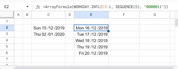
This formula follows the syntax WORKDAY.INTL(start_date, num_days, [weekend], [holidays]).
Where:
start_date:C2-1– one day before the start date in cell C2. This ensures that the sequence starts from the date in cell C2, inclusive.num_days:SEQUENCE(5)– generates sequence numbers from 1 to 5. If you specify 1, the formula will return a date after 1 day from C2-1. Here, the formula returns 5 dates excluding weekends.weekend:"0000011"– represents Saturday and Sunday as weekends. You can specify 7 0s or 1s, where 0 represents a working day and 1 represents a weekend. The order is from Monday to Sunday.
This formula paves the way to generate the sequence of working dates between two dates.
You just need to know how to replace 5, which is num_days, with a dynamic number that expands the formula to reach the end date in cell C3.
We will see that in the next step.
Step 2: Defining num_days Dynamically
To determine the number of days to specify instead of 5, we can use another date function, the NETWORKDAYS.INTL function.
This function returns the number of working days between a start date and an end date.
Syntax:
NETWORKDAYS.INTL(start_date, end_date, [weekend], [holidays])We have the start and end dates in cells C2 and C3, respectively. We also know the weekend specification, which is "0000011".
So the formula will be:
=NETWORKDAYS.INTL(C2, C3, "0000011") // returns 14Step 3: Formula to Return All Working Dates Between Two Dates
Now we just need to connect the dots. In the Step 1 formula, replace the num_days (which is 5) with the formula from Step 2.
Here it is:
=ArrayFormula(WORKDAY.INTL(C2-1, SEQUENCE(NETWORKDAYS.INTL(C2, C3, "0000011")), "0000011"))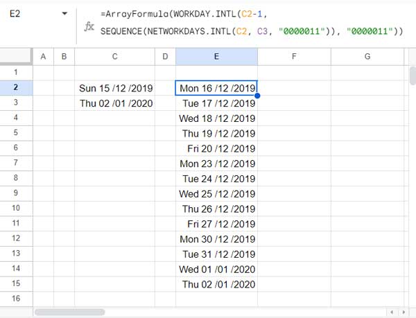
This formula will return all working dates between 2019-12-15 and 2020-01-02.
Excluding specific holidays is quite easy. We will see that next.
Return All Working Dates Between Two Dates (Excluding Holidays)
To exclude specific holidays such as New Year, Labor Day, Harvest Festival, etc., specify those dates in a column and reference that range in the formula.
The reference should be placed after the weekend specification. In our formula, we have specified weekends in two places, so you should specify the holiday reference in both places.
For example, if you have specified your holidays in D2:D4, the formula will become:
=ArrayFormula(WORKDAY.INTL(C2-1, SEQUENCE(NETWORKDAYS.INTL(C2, C3, "0000011", D2:D4)), "0000011", D2:D4))That’s all about generating a sequence of working dates between two dates in Google Sheets.
Resources
Here are some Google Sheets resources that revolve around the date sequence.
- How to Auto-Populate Dates Between Two Given Dates in Google Sheets
- Increment Months Between Two Given Dates in Google Sheets
- Elapsed Days and Time Between Two Dates in Google Sheets
- Find Missing Sequential Dates in a List in Google Sheets
- Auto-Fill Sequential Dates When Value Entered in Next Column
- How to Get Sequence of Months in Google Sheets
- Creating Sequential Dates in Equally Merged Cells in Google Sheets
- Calculate Days in Each Month Between Two Dates in Google Sheets
- Expand Dates and Assign Values in Google Sheets (Array Formula)


This doesn’t always work if the month ends on a weekend.
Hi, brad,
Thanks for pointing out the issue. We can solve that using Query.
I’ll update the post soon!