We can use a formula to find/calculate Net Working days in Google Sheets.
Many users, especially newbies, think that it’s impossible to calculate Net Working days in Google Sheets as it depends on two main factors
They are the weekends and holidays that fall between the two dates that affect the Net Workday calculation.
In India and most of the western world, Saturday and Sunday are the weekends.
That means the working days, which we want to count in Net Working days, are from Monday to Friday (excluding public holidays).
But there are countries like Israel, Iran, and Kuwait where the working days are probably from Sunday to Thursday.
Their weekend holidays are on Friday and Saturday.
Further, in some countries like India and Bangladesh, there are different working days across sectors.
Another major hurdle in Net Workdays calculation is the holidays which may not be the same every year.
But with the help of this tutorial, you can learn how to find/calculate Net Working days in Google Sheets correctly.
No matter in which country you are residing, you can follow this tutorial and correctly count Net Working days between two given dates.
Further, you can exclude or include holidays (not weekends) in the calculation.
How to Find Net Working Days in Google Sheets
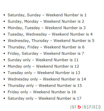
Before going to the tutorial, please take a note of the below weekend numbers.
It’s an essential part of the Net Workday calculation in Google Sheets.
If you want to perform Net Working days calculations very often, possibly if you are an HR person or working in accounts, take a note of the below numbers or bookmark this page.

To find Net Working days in Google Sheets, we can depend on the function NETWORKDAYS.INTL.
Must Read: Google Sheets Date Functions – The complete guide
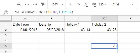
For example, I am calculating the networking days between 01/01/2018 to 05/02/2018.
I’ve chosen a shorter duration to facilitate you to manually count the days and match them with the formula result.
My default dates are in DD/MM/YYYY format. But you are OK to stick with your default date format.
To make the idea clearer to you, I am taking two countries as examples where weekends are different.
Let’s consider India and Iran here.
Net Working Days Calculations in India
Starting Date: 01/01/2018
End Date: 05/02/2018
First, let us check the official holidays during this period in India.
There are national as well as regional holidays. So as a better practice, you can stick with the holidays your company has declared.
I’m taking two holidays here as an example.
14/01/2018 – Pongal
26/01/2018 – Republic Day
Now from these inputs, we can find the Net Working days between the given two dates, which are from 01/01/2018 to 05/02/2018, both these dates inclusive.
Function Syntax: NETWORKDAYS.INTL(start_date, end_date, [weekend], [holidays])
We have the working day “start_date” and “end_date” and also the “holidays.”
To find the weekend, please check the above chart.
As you may know, in India, usually Saturday and Sunday are the weekends. So here I am considering weekend number 1.
If your office is working from Monday to Saturday, you can use the weekend number 11.
The above chart has all the weekend numbers for you to choose from. See the formula now.
=NETWORKDAYS.INTL(A2,B2,1,C2:D2)
Formula Explanation
As you can see, the Net workday start date in cell A2 and the Net Workday end date in cell B2.
As mentioned above, 1 is the weekend number for Saturday-Sunday.
In cell range C2:D2, I’ve entered the holidays not in date format but datevalue!
The NETWORKDAYS.INTL function does not support holidays as it’s. Our holidays in the example are 14/01/2018 and 26/01/2018.
You may convert it into the corresponding Date values.
In cell C2, enter the holiday as below.
=datevalue("2018/01/14")Follow the same to enter the holiday date in cell D2.
=datevalue("2018/01/26")You must stick with the above yyyy/mm/dd format in date value. Check my date function tutorial for more info. That’s all.
Update:- The function now supports dates in the holiday argument. Since, no need to convert the holidays to date values as per the above para.
Instead of giving cell references, you can use the formula as below.
=NETWORKDAYS.INTL(DATE(2018, 1, 1), DATE(2018, 2, 5), 1,{datevalue("2018/01/14"),datevalue("2018/01/26")})
=NETWORKDAYS.INTL(DATE(2018, 1, 1), DATE(2018, 2, 5), 1,{date(2018,1,14),date(2018,1,26)})
Note:- If the holiday falls on weekends, it won’t be considered twice, and that’s the beauty of this formula.
Further, if you don’t want to consider the holidays, you can exclude them in the formula as it’s optional.
Net Working Days Calculations in Iran or in Middle East Countries.
It’s another example of how to use different weekend numbers and holidays in the networking day calculation.
It’s is in line with the above Net Working days calculation in Google Sheets. The only difference is the weekend number.
Here the weekend number is 7 (Friday – Saturday).
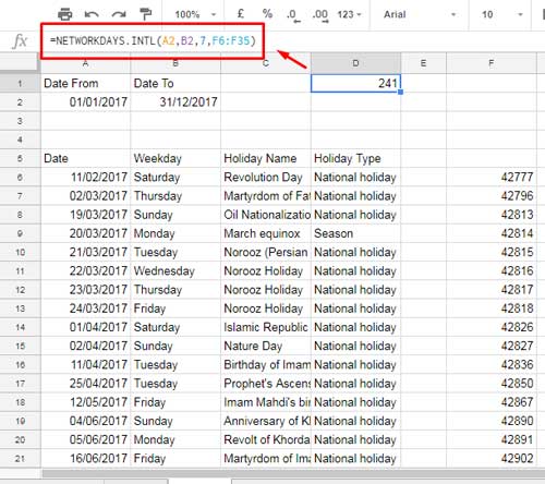
For the example, I’m considering a whole year that is from 01/01/2017 to 31/12/2017.
Please see the below screenshot.

I’ve imported a list of holidays prevailing in Iran in 2017. It may or may not be correct.
The column range A6:D35 contains the holiday’s date. But I could only capture part of the data below.
As you may know, we can’t use the date as it’s in our formula.
Update:- The function (NETWORKDAYS.INTL) started supporting dates also.
So I’ve converted it to date value using the DATEVALUE function.
The below array formula in F6 can convert all the dates in column A to the date value.
=ArrayFormula(datevalue(A6:A35))The Formula to find Net Working Days in the Middle East Based on Weekend Number 7:
=NETWORKDAYS.INTL(A2,B2,7,F6:F35)Similar: Learn the Complete TIME-related functions in Google Sheets
Conclusion
If you manually go for Net Working days calculation, there are chances of error.
If an employee has worked for more than one year, you may find it difficult to count the Net Working days; manually.
So learn NETWORKDAYS.INTL function and also thorough weekend numbers.
I guess, with the help of this tutorial, you may be able to learn how to find Net Working Days in Google Sheets.
Thanks for the stay. Enjoy!
Related:-


