Counting values between two dates or within date ranges is a broad topic. You can use different functions or function combinations in Google Sheets depending on your purpose.
For example, you may want to count all or specific values within a date range. There could be more than two columns or rows involved. Based on that, we select our functions or combinations.
Let me start with a basic example, where I’ll use the COUNTIFS function to achieve my goal.
Counting Values Between Two Dates in Google Sheets
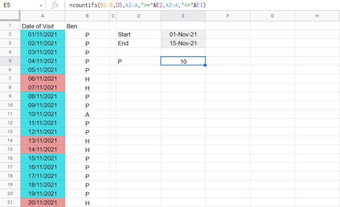
I want to count the number of “P” (present) within the date range 01/11/2021 to 15/11/2021. The dates are in column A, and the statuses (“P”) are in column B.
Here, we want to count a specific value between two dates.
Formula:
=COUNTIFS(B2:B, "P", A2:A, ">="&DATE(2021,11,1), A2:A,"<="&DATE(2021,11,15))In the formula above, the criteria are the dates 01/11/2021 and 15/11/2021 as per the syntax DATE(year, month, day), and the string “P.”
We can specify these criteria in cells and use the following formula:
=COUNTIFS(B2:B, D5, A2:A, ">="&E2, A2:A, "<="&E3)Where D5 contains “P”, E2 contains the start date of the range, and E3 contains the end date of the range.
To count all values between two dates, replace the specific value “P” or the reference D5 in the above formulas with the wildcard “*” (asterisk):
=COUNTIFS(B2:B, "*", A2:A, ">="&E2, A2:A, "<="&E3)The real challenge arises when the values are spread across multiple rows and columns.
Counting Values Across Multiple Columns Between Two Dates
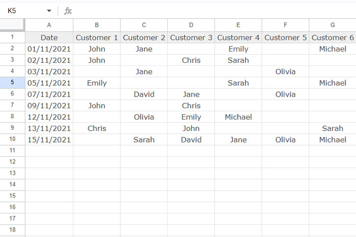
Assume you maintain your call logs for payment follow-ups in a table. The dates are in column A (A2:A), and customer names are in columns B to G (B2:G).
The purpose of multiple columns is to record all calls made on a specific day, avoiding the need to repeat the dates in multiple rows.
How do you count the number of calls made to a specific customer or all customers during a specific period?
The following examples show how to count values across multiple columns that fall between two dates in another column.
Example 1: Counting Calls for a Specific Customer During a Period
The following COUNTIFS formula will count the number of times the customer name “Olivia” appears in the range B2:G between the dates 01/11/2021 and 10/11/2021 in A2:A:
=COUNTIFS(FILTER(B2:G, A2:A>=DATE(2021, 11, 1), A2:A<=DATE(2021, 11, 10)), "Olivia")The FILTER function filters the range B2:G based on the conditions where A2:A is greater than or equal to the start date and less than or equal to the end date.
It follows the syntax: FILTER(range, condition1, [condition2, …])
Where:
range:B2:G– the range to filter.condition1:A2:A >= DATE(2021, 11, 1)condition2:A2:A <= DATE(2021, 11, 10)
The COUNTIFS function then counts the occurrences of the customer name “Olivia” within this filtered range.
Example 2: Counting Calls for All Customers During a Period
In the previous example, we counted specific values in multiple columns between two dates. In this example, we will count all values.
We will first filter the data as before. Instead of applying COUNTIFS, we will use TOCOL to arrange the data into a single column and then use QUERY to aggregate it.
=QUERY(TOCOL(FILTER(B2:G, A2:A>=DATE(2021, 11, 1), A2:A<=DATE(2021, 11, 10)), 3), "SELECT Col1, COUNT(Col1) GROUP BY Col1 LABEL COUNT(Col1)''", 0)Result:
| Chris | 2 |
| David | 1 |
| Emily | 2 |
| Jane | 3 |
| John | 3 |
| Michael | 2 |
| Olivia | 2 |
| Sarah | 2 |
If you are not familiar with QUERY, don’t worry. Just replace the filter part with your FILTER formula. The rest of the formula will handle the aggregation for you.
Resources
- COUNTIFS in a Time Range in Google Sheets [Date and Time Column]
- COUNTIF to Count by Month in a Date Range in Google Sheets
- Count Unique Dates in a Date Range – 5 Formula Options in Google Sheets
- How to Count Events in Particular Timeslots in Google Sheets
- Countdown Timers in Google Sheets (Easy Way!)


Thanks for all your contributions to helping people to familiarize themselves with Google Spreadsheets.
This example is really cool. I just have one question, how we can use the same idea, but when the start and end date are an array of values.
Thanks.
Hi, David Leal,
I’m glad to know that you find my Google Sheets tutorials useful.
Regarding your query, can you please make a sample sheet? You can share the URL of the same in your reply below. I will keep it unpublished.