You can count the months and days between two dates using the QUERY or DATEDIF function in Google Sheets.

Use either of them, depending on your purpose.

1. DATEDIF:- Require two formulas based on this function to get the required output.
   1. Use one formula (the unit is ‘M’) to return whole months between dates.
   2. Another (‘MD’) to get the balance/remaining days.
2. QUERY:- Its purpose is entirely different here. We can use this function to list the months in one column and the corresponding number of days in another column.

As you may already know, there are several date-related functions in Google Sheets. DAYS, NETWROKDAYS, and the DATEDIF are a few of them.

These built-in functions allow users to calculate the number of days, weeks, years, networking days, etc., from a start date and end date.

But as far as I know, there is no native Google Sheets function to get the number of days and months between two dates in one go!

Whole Months between Dates and Balance Days Using the DATEDIF Function in Google Sheets

What is a whole month in the DATEDIF function in Google Sheets?

Let’s try to understand it with an example.

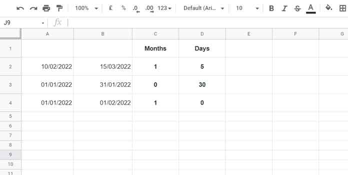
Note:- The formats of the below values in cells A2 and B2 are in DD/MM/YYYY format.

A2: 10/02/2022

B2: 15/03/2022

To calculate the months between these two dates and the remaining days, we can use the following formulas in cells C2 and D2, respectively.

=datedif(A2,B2,"M")

Output = 1

=datedif(A2,B2,"MD")

Output = 5

The first formula counts 28 days from 10/02/2022, i.e., up to 10/03/2022.

It’s because the starting date falls in February, which has 28 days.

The second formula returns the remaining days, i.e., 5, from 11/02/2022 to 15/02/2022.

This way, we can get whole months between dates and remaining days in Google Sheets.

In the above examples (please refer to the image above), the given formulas in cells C2 and D2 are dragged down. Check their outputs in columns C and D to get a clear picture.

Now let’s see how the above DATEDIF differs from the QUERY-based solution.

Query to Return the Months and Actual Days between a Start and End Date

I have two formulas using the Query function here.

One is a basic formula that doesn’t come with formatting. Please refer to column D in the screenshot below.

Basic Formula (in D1):

=ArrayFormula(
     query(
        to_date(row(indirect("A"&A2):indirect("A"&B2))),
        "Select month(Col1)+1,count(Col1) group by month(Col1)"
     )
)

I don’t advise using the above basic formula as it has one drawback. What’s it?

If your start and end dates fall in two different years, it won’t work correctly.

The second formula in cell G1 is highly formatted and without the said drawback.

It returns proper field labels, and unlike the D1 formula, the months are in text format like January, February, etc. Please refer to column G (screenshot) below.

Suggested Formula (in G1):

=ArrayFormula(
     query(
        EOMONTH(row(indirect("A"&A2):indirect("A"&B2)),0),
        "Select Col1, Count(Col1) group by Col1 label Col1 'Month',
        count(Col1)'Days in Month' format Col1'MMMM-YYYY'"
     )
)

See both the results. That can help you to choose the Query formula that you want.

This way, we can use Query to return the months and actual days between a start and end date in Google Sheets.

Formula Explanation (Query)

Let me start with the D1 formula.

In Google Sheets, a date is a number formatted to date. Do you want to test it?

To get that number, you can use the DATEVALUE function as below (feel free to refer to my Google Sheets Functions Guide to learn it).

=datevalue(A2)

Result: 43158

=datevalue(B2)

Result: 43192

The above are the actual values in cells A2 and B2. Now see the below ROW formula.

=ArrayFormula(row(43158:43192))

This formula would return the (sequential) numbers from 43158 to 43192 row-wise. These are actually the dates from 27/02/2018 to 02/04/2018.

You can use the function TO_DATE to format the above numbers back to dates.

=ArrayFormula(TO_DATE(row(43158:43192)))

Since we have the values in cells A2 and B2, I’ve used the function Indirect to get them in the Row formula. Without using Indirect, the D1 formula would look like this.

=ArrayFormula(
     query(
        TO_DATE(row(43158:43192)),
        "Select month(Col1)+1,count(Col1) group by month(Col1)"
     )
)

The Query is used to group the dates by month and return the count.

Why have I used month(Col1)+1 in the formula?

The Query returns the month number from 0 to 11 instead of 1 to 12. The +1 solves this puzzle.

What about the G1 formula?

I have used EOMONTH instead of TO_DATE in comparison to the D1 formula and the Format clause additionally.

That’s as per tutorial # 2 under the “Resource” below.

I hope the above formulas help you find months and days between two dates in Google Sheets.

Thanks for the stay. Enjoy!

Resources

1. How to Convert Month in Number to Month Name in Text.
2. How to Group Data by Month and Year in Google Sheets.
3. Increment Months Between Two Given Dates in Google Sheets.
4. Array Formula to Lookup Date Between Two Dates in Google Sheets.
5. Elapsed Days and Time Between Two Dates in Google Sheets.
6. Return All Working Dates Between Two Dates in Google Sheets.
7. Count Values Between Two Dates in Google Sheets.