With a built-in function, we can unique rows ignoring date-times in a timestamp column in Google Sheets.

To your surprise, the function is SORTN, not UNIQUE.

If you use the UNIQUE for the said purpose, you may use an additional VLOOKUP function.

I have included both the solutions and some extra tips and tricks to make this tutorial worthy for you to read.

Introduction

If you are using Google Docs Form for collecting information, you may find the tips on this tutorial useful.

If someone submits an entry in your form, the record may contain a timestamp of it. In a connected Sheet, the first column will be the Timestamp column.

If a person posts multiple entries with the same data, then you may have duplicate records in your connected sheet.

One of the obstacles to removing such duplicate rows in Google Sheets will be the Timestamp column. You may require to find a way to unique rows ignoring the timestamps.

To remove duplicate rows from such data, I mean to unique rows ignoring the Timestamp column, we can use the SORTN function in Google Sheets.

From my point of view, it’s the easiest solution for this purpose.

Let’s straightaway go to an example.

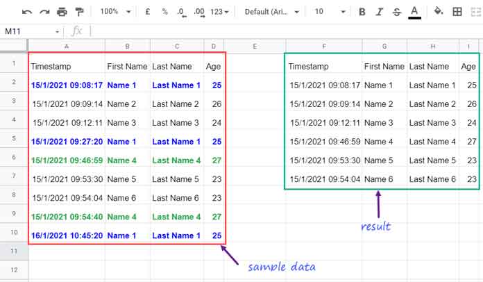
Sample Form Entries in a Connected Sheet:

Sample Data in A1:D10 and expected result in F1:I7.

Unique Rows Ignoring Timestamp Column in Google Sheets

If you use the UNIQUE function to wrap the data in A2:D10, the formula will return the range as it is.

=unique(A1:E10)

As I have mentioned, it’s due to the timestamps in column A.

Can I use the Unique function to remove duplicate rows ignoring the timestamp column in Google Sheets?

Yes! We can. But we need an additional formula. Find them below.

UNIQUE and VLOOKUP Approach (Workaround Method)

Even though I am not recommending this formula, I include it to show you the capability of Google Sheets.

The following formula in cell G1 will return the required output in G1:I7. You may refer to the image above.

=unique(B1:D10)

It’s at the cost of the Timestamp column.

To get the timestamp column, use the following Vlookup array formula in cell F1.

=ArrayFormula(vlookup(G1:G7&H1:H7&I1:I7,{B1:B10&C1:C10&D1:D10,A1:D10},2,0))

So you will get the same output as shown in the above image.

Using a simple SORTN formula, we can unique rows ignoring a Timestamp column in Google Sheets.

Since the timestamps are involved, you can decide which form entry to be considered – the first one or the last one.

I mean, when a user submits multiple entries via Form, you can keep the first one or the last one based on your choice.

SORTN Approach (Recommended)

First Form Entry

We can replace the above Vlookup in cell F1 and Unique in cell G1 with a single SORTN formula in cell F1.

=sortn(A1:D10,9^9,2,B1:B10&C1:C10&D1:D10,1)

This will return the same result shown in the above image.

That means the formula keeps the first entry from a user, and other records submitted by him got removed.

In concise, we can read the above SORTN formula as below.

A1:D10 – Data range

9^9 – An arbitrarily large number (maximum number of rows in the output)

2 – Remove duplicates

B1:B&C1:C&D1:D – All the columns combined except the Timestamp column. The formula unique the rows ignoring the timestamp column based on it.

1 – Sort the result based on the above-combined columns in ascending order.

Using the above SORTN in an open range may cause a blank row at the top of the result. In such a case, we can use FILTER or QUERY to remove that row. I am using Query.

Note:- A1:A10 is a closed range, whereas A1:A is an open range.

Formula in F1:

=Query(sortn(A1:D,9^9,2,B1:B&C1:C&D1:D,1),"Select * where Col1 is not null")

Last Form Entry

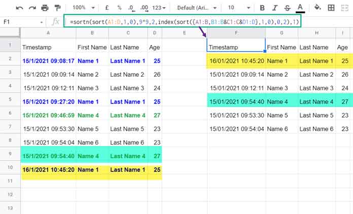
See the below formula output and compare its output with the source data in A1:D.

Formula in F1:

=sortn(sort(A1:D10,1,0),9^9,2,index(sort({A1:A10,B1:B10&C1:C10&D1:D10},1,0),0,2),1)

As you can see, the formula retains the last form entry.

It’s made possible by sorting the timestamp column in descending order that within the formula itself.

I mean replaced A1:D10 with sort(A1:D10,1,0) and B1:B10&C1:C10&D1:D10 with index(sort({A1:A10,B1:B10&C1:C10&D1:D10},1,0),0,2).

Here also use the QUERY to sort out the blank row in an open range.

=query(sortn(sort(A1:D,1,0),9^9,2,index(sort({A1:A,B1:B&C1:C&D1:D},1,0),0,2),1),"Select * where Col1 is not null")

This way, we can unique rows ignoring a Timestamp column in Google Sheets.

Unique Rows Ignoring Timestamp Column Plus One More Column

Before concluding this tutorial, let me clarify one more thing.

You can consider a few columns as above to unique a table. In the above example, I have taken the columns “First Name”, “Last Name”, and “Age”.

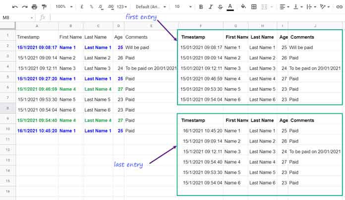
Assume I have one more column labeled as “Comments”. The user may enter the same comment or a different comment in every new form submission.

So this time, you may have to ignore both the Timestamp and Comments column. So the formula will be,

First Entry;

=Query(sortn(A1:E,9^9,2,B1:B&C1:C&D1:D,1),"Select * where Col1 is not null")

Last Entry;

=query(sortn(sort(A1:E,1,0),9^9,2,index(sort({A1:A,B1:B&C1:C&D1:D},1,0),0,2),1),"Select * where Col1 is not null")

I hope you could understand how to unique rows excluding timestamp column in Google Sheets.

Thanks for the stay. Enjoy!