One powerful and flexible way to look up values is by combining the OFFSET and MATCH functions in Google Sheets. While there are many other options available, let’s explore why this combination stands out.
In this approach, we’ll use MATCH to search for a value and OFFSET to return a value or an array from that point. Additionally, we can use multiple matches to extract rows between two points by dynamically specifying the height of the rows to return.
OFFSET and MATCH Regular Use Case
First, let’s take a look at the syntax for the OFFSET function:
OFFSET(cell_reference, offset_rows, offset_columns, [height], [width])The OFFSET function allows you to offset rows and columns from a specified point, with optional parameters for height and width.
For example, consider the sample data in the range B2:J10 below. The following formula will return the value from cell B5 by offsetting 3 rows (i.e., B2, B3, and B4) from the starting point in cell B2.
=OFFSET(B2, 3, 0, 1, 1)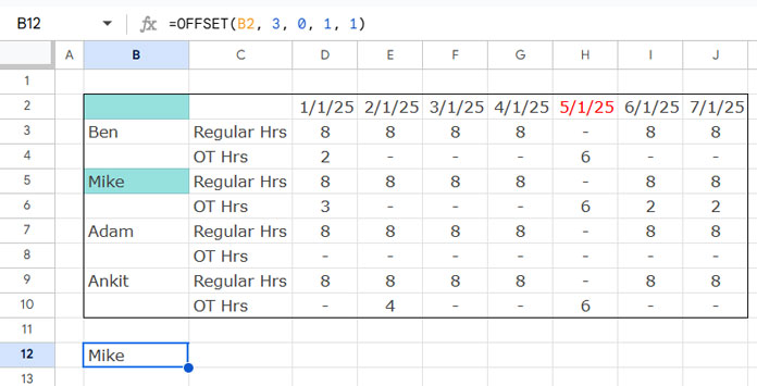
Here, the offset for the columns is 0, meaning it returns the value from the same column, and both the width and height are set to 1 cell.
To dynamically specify the row offset, you can replace the offset_rows with a MATCH formula like this:
MATCH("Mike", B2:B10, FALSE)-1This formula matches the name “Mike” in the range B2:B10 and returns the relative position (in this case, 4, as “Mike” is in the fourth row of the range). Since OFFSET starts counting from 0, we subtract 1 from the MATCH result.
So, the final formula using both OFFSET and MATCH in Google Sheets is:
=OFFSET(B2, MATCH("Mike", B2:B10, FALSE)-1, 0, 1, 1)In practice, there’s no need to search for the name “Mike” just to return the name itself. Instead, you can specify a different column offset to return data from another column.
For example:
=OFFSET(B2, MATCH("Mike", B2:B10, FALSE)-1, 2, 1, 1)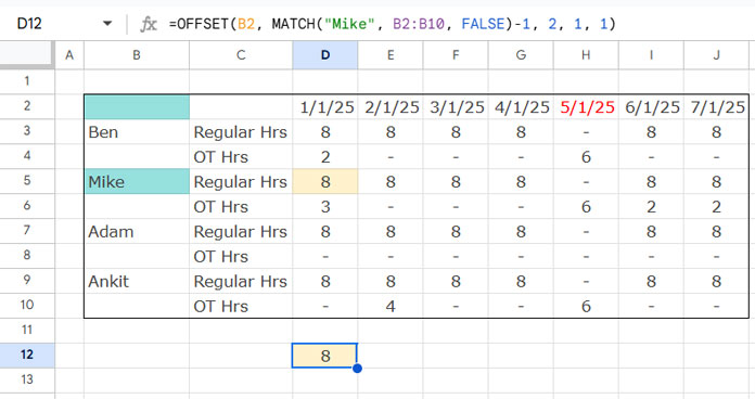
This will return the normal hours for Mike on 1/1/25. If you want to return both regular and overtime hours, specify a height of 2:
=OFFSET(B2, MATCH("Mike", B2:B10, FALSE)-1, 2, 2, 1)To return two rows and seven columns (for example, hours for multiple dates), use the following formula:
=OFFSET(B2, MATCH("Mike", B2:B10, FALSE)-1, 2, 2, 7)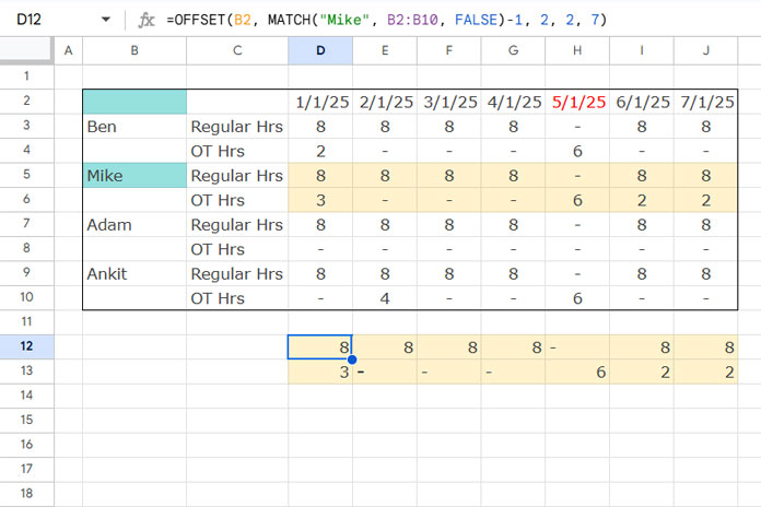
This demonstrates how using OFFSET with MATCH in Google Sheets differs from regular lookup functions like VLOOKUP, XLOOKUP, etc.
Using OFFSET and MATCH to Extract Rows Between Two Values in a Column
Approach 1
In the previous example, we specified the width as 2 to return both regular and overtime hours for Mike. You can achieve the same output by using MATCH to find the rows between two values, like “Mike” and “Adam.”
First, calculate the row offset for “Mike” using:
MATCH("Mike", B2:B10, FALSE)-1Next, calculate the height as the difference between the positions of “Adam” and “Mike”:
MATCH("Adam", B2:B10, FALSE)-MATCH("Mike", B2:B10, FALSE)Now, use the following formula to extract the rows between “Mike” and “Adam”:
=OFFSET(B2, MATCH("Mike", B2:B10, FALSE)-1, 2, MATCH("Adam", B2:B10, FALSE)-MATCH("Mike", B2:B10, FALSE), 7)This will return the rows between the two names.
Approach 2
In the previous example, we used MATCH("Adam", B2:B10, FALSE)-MATCH("Mike", B2:B10, FALSE) to calculate the height. You can replace this with a more advanced formula to make it more dynamic:
MATCH("Adam", OFFSET(B2, MATCH("Mike", B2:B10, FALSE)-1, 0, 5, 1), FALSE)-1The full formula is:
=OFFSET(B2, MATCH("Mike", B2:B10, FALSE)-1, 2, MATCH("Adam", OFFSET(B2, MATCH("Mike", B2:B10, FALSE)-1, 0, 5, 1), FALSE)-1, 7)This will yield the same output as in Approach 1. However, this method is more precise in some cases, as it ensures “Adam” is matched after “Mike”. If “Adam” appears both before and after “Mike”, the first formula (approach 1) will return a #VALUE error.
Explanation (height):
OFFSET(B2, MATCH("Mike", B2:B10, FALSE)-1, 0, 5, 1)In this OFFSET and MATCH combination, MATCH is used to find the position of “Mike” in column B. OFFSET then shifts that many rows, extracting 5 rows from the range (you can use 5 or a larger number, depending on your data, as the goal is to extract all the values below “Mike”).
We then use this output as the range for another MATCH formula to find the position of “Adam” and return the relative position.
MATCH("Adam", ..., FALSE)-1


