You don’t like to remove duplicates manually. It’s time-consuming and error-prone, right?

This post is a gateway to a few walkthrough guides that can help you learn how to remove duplicates in Google Sheets.

We have a wide variety of options in hand to find and remove duplicates in Google Sheets.

Depending on your data type, your requirements may vary.

The formula one user finds suitable for him may not be idle for another user because of the datatypes he handles.

I have already coded a few formulas and a custom function for this specific purpose.

Also, you can depend on the Data > Data clean-up command.

You can find two sections in this post: One is how to remove duplicates, and the other is how to find duplicates.

Formulas to Remove Duplicates Rows in Google Sheets

1. Removing Identical Rows and Columns: UNIQUE

This is is the easiest method to remove duplicates in Google Sheets.

The UNIQUE function is suitable for removing duplicates in a single column.

=unique(A2:A7)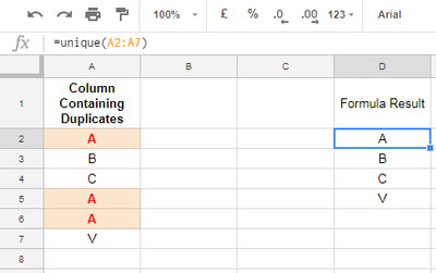

But if you want to remove duplicates in multiple columns, this function works in a limited way.

In the following example, the character “A” repeats thrice in column A. But the third occurrence is not a duplicate as its value in the second column is different.

=unique(A2:B7)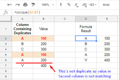

Detailed Tutorial: Removing Duplicates Using Unique in Google Sheets.

2. Get Unique Rows Based on Distinct Column(s): SORTN

How to operate a particular column to find and remove duplicates? Of course, UNIQUE isn’t capable doing this.

The solution is the SORTN function with display tie mode # 2.

SORTN is something that you should learn to get unique rows based on a distinct column in Google Sheets.

For example, if your table contains the name (A1:A) and email address (B1:B) of students in two columns and remove duplicates based on the email column, then use SORTN, not UNIQUE.

Unique by Distinct One Column:

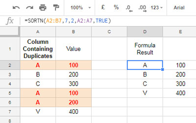
=sortn(A2:B7,7,2,A2:A7,TRUE)

The above Google Sheets formula returns unique rows based on the distinct range A2:A7.

range: A2:B7

Number of rows to return: 7 (specify total rows or 9^9, an arbitrarily large number)

Display ties mode: 2

Distinct by column or range: A2:A7

Sort: TRUE (Asc)

Unique by Distinct Two Columns:

The following formula answers how to unique a dataset by distinct two columns in Google Sheets.

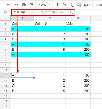
=sortn(A2:C7,10,2,A2:A7&B2:B7,TRUE)

The above Google Sheets formula returns unique rows based on the distinct range A2:A7 and B2:B7.

range: A2:C7

Number of rows to return: 10 (specify any number greater than or equal to the total rows in the range or 9^9, an arbitrarily large number)

Display ties mode: 2

Distinct by column or range: A2:A7&B2:B7

Sort: TRUE (Asc)

Read more about this killer function to remove duplicates in my following walkthrough.

Detailed Tutorial: Remove Duplicate Rows Based on Selected Columns in Google Sheets

3. Remove Duplicate Rows in Google Sheets: A Custom Function and Other Options

If you can’t find a proper solution to your problem, do not tear your hair out.

I’ve coded a few more formulas that might help you remove duplicates from your dataset. Here are them.

1. Remove Duplicate Rows and Keep The Rows With Max Value.
2. Compare Two Tables and Remove Duplicates.
3. How to Remove Duplicate Values without Deleting the Rows.
4. Remove Duplicates from Comma-Delimited Strings.
5. Removing Duplicates by Key Column (Custom Function).
6. Finding Duplicates in New Lines Inside Cells in Google Sheets.

Please let me know in the comment section below if the above still doesn’t meet your requirement.

Remove Duplicates in the Source Range Itself: Menu Command

We have come across several formulas above. All of them return the result in a new range.

They will be handy when you don’t want to touch your source data.

If you don’t want to try them, use the Remove Duplicated menu command.

Please don’t forget to back up your data beforehand.

Detailed Tutorial: Removing Duplicates Using Data Clean-up Menu in Google Sheets.

Formulas to Find and Mark Duplicate Rows in Google Sheets

1. One Distinct Column

First of all, please note that it’s a non-array formula.

So, based on our example, you should copy-paste the Countif formula in cell D2 down as far as you want.

This formula helps you to find duplicates in Google Sheets based on a distinct column.

It leaves an “X” mark wherever repeated items appear in corresponding rows in column A.

=if(countif($A$2:$A2,$A2)=1,,char(10005))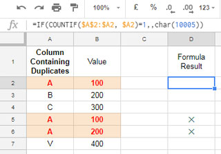

If you prefer, you can use the following array formula instead of the above one.

Empty the range D2:D and insert the below running count-based formula in cell D2.

=ArrayFormula(if(countifs(row(A2:A),"<="&row(A2:A),A2:A,A2:A)>1,char(10005),))

2. Two Distinct Columns

It’s easy to modify the above formula to apply it to two distinct columns.

The non-array formula uses the COUNTIFS function.

=if(countifs($A$2:$A2,$A2,$B$2:$B2,$B2)=1,,char(10005))

This formula would only put the “X” mark in D5 as it’s the only row that repeats.

Here is the array alternative that sits in cell D2 and spills down.

=ArrayFormula(if(A2:A="",,if(countifs(row(A2:A),"<="&row(A2:A),A2:A&B2:B,A2:A&B2:B)>1,char(10005),)))