In Google Sheets, the Data menu > Data validation is the only built-in way to reject the entry of certain values in a cell or range of cells. In this tutorial, I’m going to elaborate on how to reject a list of items in data validation in Google Sheets.

I’ve tried to shorten the title of this tutorial as much as I can. Actually, I am going to explain two data validation tips in this post. Here are them.

1. Data validation to reject/restrict a list of items (item codes, item numbers, names, or any value) in a range.
2. Rejecting a list of items if it is already available/present in another sheet or another range.

You can learn more about these two types of data validation from the following examples.

How to Reject a List of Items Using Data Validation

There are two examples (two data validation rules as per points # 1 and 2 above).

In the first example, I’ll apply the data validation settings to column A (A1:A). In the second one, the settings will go to column B (B1:B). Please note that both are in “Sheet1”.

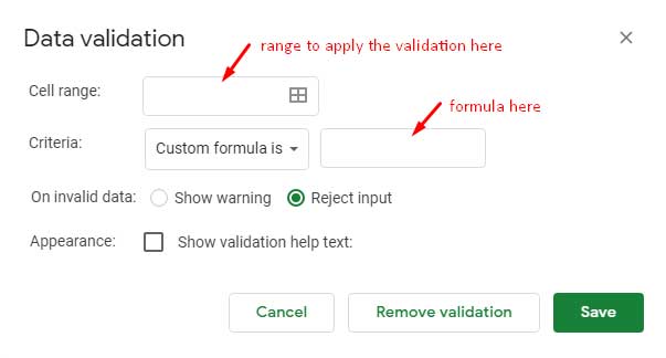
My formulas should be entered in Data > Data validation > Custom formula is field as below.

Enter the range A1:A against “Cell range” for formula 1 and B1:B for formula 2. Both the formulas you will get under the relevant subtitles below.

Let me elaborate on how to reject/block/restrict a list of items in data validation in Google Sheets.

Block (Reject Input of) a List of Values

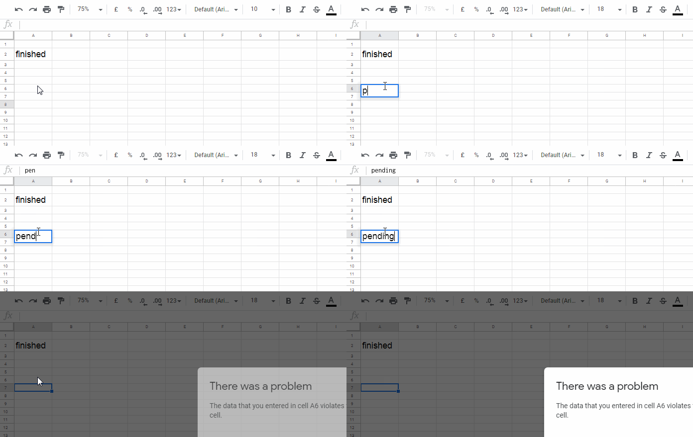
Assume I want to reject the input of the values “pending”, “withheld”, or “amended” in column A. Here is the formula (data validation rule) to do this.

Formula # 1:

=not(REGEXMATCH(to_text($A1),"pending|withheld|amended"))

The Regexmatch formula matches the strings “pending”, “withheld”, and “amended” and returns FALSE if there is no match. The outer NOT function makes the FALSE TRUE.

When the formula returns TRUE such entries are allowed in the corresponding cell in column A, else get blocked/rejected.

You can use any string, number, a list of strings as above, or a list of numbers (as below) instead of the above three strings. When there is more than one value to match, separate them by the Pipe.

Example:

"15001|15002|15003|15004"

For the exact match (the above is a partial match, that means “pending” as well as “pending work” will be rejected) use the expression as below.

"^pending$|^withheld$|^amended$"

I have used the function To_text to make the validation formula compatible for both numbers and strings.

Block (Reject Input of) a List of Values if Available in Another Sheet

Let’s address the same above scenario from an entirely different angle. In the above formula, we have tried to exclude/bar the entry of certain values in column A.

This time I want to block or reject the input of the said values in column B if those values are available in another range. That means compared to formula # 1, here a condition is involved in reject input.

Here the validation settings are for column B (Sheet1). The validation rule should block the entry of the values “pending”, “withheld”, or “amended” if they are present in any range in “Sheet2”.

Any range can be a cell (e.g. Sheet2!$A$1), any particular range (e.g. Sheet2!$A$1:E$10) or the entire “Sheet2” (e.g. Sheet2!$1:$1000, i.e. 1000 rows).

Formula to reject a list of items in column B, if it’s present in another sheet, i.e. in Sheet2!$A$1:E$10, in data validation in Google Sheets.

Formula # 2:

=REGEXMATCH(
     to_text($B1),"pending|withheld|amended"
)*
ArrayFormula(
     SUM(REGEXMATCH(to_text(Sheet2!$A$1:E$10),$B1)*1)
)=0

How the above formula blocks a list of values if it’s available in another sheet?

Formula Explanation

There are two parts in formula # 2 – one starting with the Regexmatch and the other starting with the ArrayFormula.

The first part, i.e. REGEXMATCH(to_text($B1),"pending|withheld|amended", matches the strings “pending”, “withheld”, and “amended” in cell B1 in “Sheet1”, which is in the sheet that contains the validation rule.

It returns TRUE if matches else returns FALSE (TRUE is equal to the number 1 and FALSE is 0).

The second part, i.e. ArrayFormula(SUM(REGEXMATCH(to_text(Sheet2!$A$1:E$10),$B1)*1)), matches the string in cell B1 in “Sheet1” in the range A1:E10 in “Sheet2” and returns TRUE if matches else it returns FALSE.

Actually, the Regexmatch in this second part returns an array of TRUE/FALSE values. So the SUM function has been used to return the sum of TRUE values.

So if the cell B1 value is available in “Sheet2”, the output of the second part formula would be a number greater than 0.

Our above validation rule to reject a list of items if available in another sheet in data validation can be read as below.

=part_1_formula*part_2_formula=0

This means if the cell B1 value matches in “Sheet2” then the output would be greater than 0. The rule only allows entry if the output is 0.

Formula tests;

formula_logic;
= 1 * 0 = 0 ? TRUE (match in Sheet1, not in Sheet2); permitted.
= 0 * >=1 = 0 ? TRUE (match in Sheet2, not in Sheet1); permitted.
= 1 * >=1 = 0 ? FALSE (match in Sheet1 and Sheet2); blocked.

Similar to formula # 1, here also you can apply the exact match. In the part 1 formula, you may please follow the formula # 1 explanation. For part 2, the expression $B2 should be used as "^"&$B2&"$".

That’s all about how to reject a list of items in data validation in Google Sheets. Thanks for the stay! Enjoy!

Resources

1. Data Validation – How Not to Allow Duplicates in Google Sheets.
2. The Best Data Validation Examples in Google Sheets.
3. Proper Way to Use Currency Formatting in Data Validation Drop-Down in Google Sheets.
4. Restrict Users from Entering Special Characters in Google Sheets (Data Validation).
5. Restrict or Force Text Entry to All Caps, All Lower Case, or Proper Case.
6. Restrict People from Entering Invalid Data on Google Doc Spreadsheet.