Currency formatting can cause two types of issues in the data validation drop-down list in Google Sheets.

1. Violation of data validation rules.
2. Invalid number formatting (numbers/currency formatted as text).

Here are some simple steps to sort out the number/currency formatting associated issues when using numbers in the data validation drop-down lists in Google Sheets.

For example, let’s consider a column contain drop-down lists that permit me to select the numbers from 1 to 10. I want to use these numbers as the unit rate of items so I want currency formatting applied to these numbers.

When I choose any number, for example, the number 5, I want to get it formatted as $5, not as an unformatted number 5.

That, of course, I can do with number formatting and would probably work correctly in Google Sheets. But some times it can cause a data validation rule violation. I’ll come to it.

In another scenario, when I choose $5 from a drop-down list contains $1 to $10, I want to get it as $5, in number format, not in text format.

Here are the proper ways to use currency formatting in the data validation drop-down list in Google Sheets.

Currency Formatting in Data Validation Drop-Down Using List of Items Method in Google Sheets

In the “Lst of items” method, there are two ways to use currency/number formatting in a drop-down list in Google Sheets. Find that below.

Number Formatting the Drop-Down List Using Custom Number Format

In this method, I will create the drop-down lists as shown in the image below. As you can see I have used only unformatted numbers. I mean there are no currency signs with numbers.

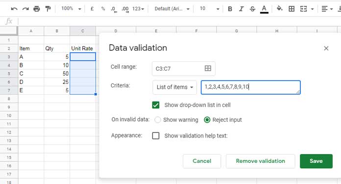
It will create a drop-down in the range C3:C7. Select the range C3:C7 and format it as ‘Currency’ from the Format menu in Google Sheets.

Note: It’ll only format the range with default currency sign. If your default currency and currency that you want are different, then instead of Format > Number > Currency, use Format > Number > More formats > More currencies to format the range C3:C7.

Click any drop-down, for example, cell C3, and select any number. You will see the following error.

The data you entered in cell C3 violates the data validation rules set on this cell. Please enter one of the following values: 1, 2, 3, 4, 5, 6, 7, 8, 9, 10.

To use currency formatting in such type of data validation list in Google Sheets, do as follows.

1. Select the range C3:C7 which contains the drop-down lists.
2. Go to Data > Data validation.
3. Against “On valid data” settings, enable “Show warning” and Save the settings.

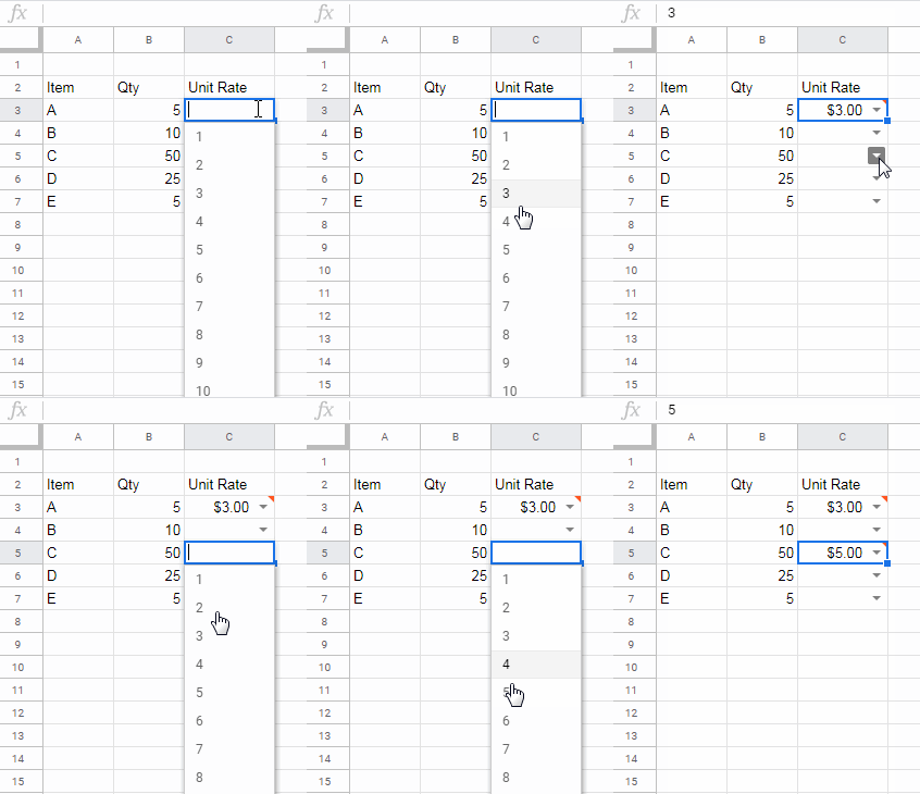
Simply ignore the warning.

Include the Currency Sign within List of Items

Some users follow the below method to get currency formatting in data validation drop-down in Google Sheets. It has two drawbacks though.

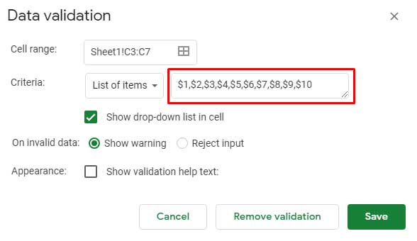
What are they (drawbacks)?

Different Default Currency

If your sheets’ default currency and the currency used in the list of items are different, the numbers (currency) will be treated as text. So won’t work in calculations.

For example, my sheets’ default currency (the currency sign that I get by applying Format > Number > Currency) is £ (British Pound Sterling).

Since I have used the $ (US Dollar) within ‘List of items’ in data validation, it converts the number to text. So obviously the formula in cell D3 would return the #VALUE! error.

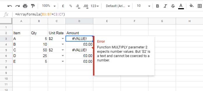
Here to solve the error, you may need to change the default currency by changing the ‘Locale’ from within the File menu ‘Spreadsheet settings’.

Same Default Currency

Here is the drawback # 2.

Even if the currency signs are the same (the default currency and the currency used in the ‘List of items’), you can’t use the 1000 separator. So using a number with more than 3 digits won’t be possible.

The number formatting like $5000 will work, but won’t $5,000 because the comma will be treated like a number separator, not like a thousand separator in data validation.

Currency Formatting in Data Validation Drop-Down Using List from Range Method in Google Sheets

The proper way to use currency formatting in the data validation drop-down list in Google Sheets is the “List from range” method in data validation.

In this keep the numbers (plain numbers) as a list in another column and use it in data validation. Then custom number format the drop-down list with the required currency sign.

Here are the steps involved.

• I have the list in G2:G11 which contains the numbers 1 to 10.
• Select C3:C7 and go to Data > Data validation.
• Against the Criteria “List from a range”, select G2:G11 and “Save”.
• Format C2:C7 using Format > Number > More formats > More currencies.

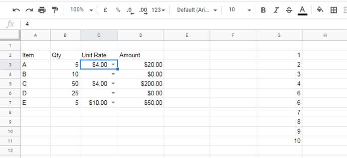
This is the simple and correct method to format numbers in a drop-down list to currency in Google Sheets.

That’s all. Enjoy!

Data Validation Resources

• Data Validation – How Not to Allow Duplicates in Google Sheets.
• The Best Data Validation Examples in Google Sheets.
• Multi-Row Dynamic Dependent Drop Down List in Google Sheets.
• A Drop-down Menu in Google Sheets to View Content from Any Sheets in the Current Sheet.
• Auto-Populate Information Based on Drop-down Selection in Google Sheets.
• Distinct Values in Drop Down List in Google Sheets.
• Google Sheets: How to Get an All Selection Option in a Drop-down.
• Populate a Full Month’s Dates Based on a Drop-down in Google Sheets.
• Create a Drop-Down to Filter Data From Rows and Columns.
• Create a Drop-Down Menu From Multiple Ranges in Google Sheets.
• How to Combine Multiple Sheets in Importrange and Control Via Drop-Down.