How to Use Column Headers in Google Sheets QUERY (2 Dynamic Methods)

You can’t directly use column headers (field labels) in the Google Sheets QUERY function. This becomes a problem when columns are inserted or moved, as QUERY relies on position-based references. However, there are two dynamic methods you can use as workarounds: using LET to assign names to columns and using table references.

Before diving into these methods, it’s important to understand the benefit of using column headers in QUERY.

Table of Contents

Why Use Column Headers in Google Sheets QUERY?

The QUERY function supports two types of column identifiers:
letters such as A, B, …, Z, AA, AB, …, or Col1, Col2, …, Col26, Col27, Col28, ….

However, QUERY does not inherently recognize columns by their headers. For example, if your data is in the range B2:D and the headers in B2, C2, and D2 are “Name,” “Dept,” and “Salary,” you cannot write:

=QUERY(B2:D, "SELECT Dept", 1)

Instead, you must use:

=QUERY(B2:D, "SELECT C", 1)
=QUERY(B2:D, "SELECT Col2", 1)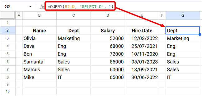

Google Sheets QUERY selecting a column using column letter C instead of header

The real issue arises when you insert new columns into the dataset. Since these identifiers are position-based, your formulas won’t adjust automatically and may return incorrect results.

This tutorial shows how to reference columns using field labels (headers) in the Google Sheets QUERY function, so your formulas remain dynamic and robust.

Method 1: Using LET to Reference Column Headers in QUERY

Let’s start with an example.

The following formula selects the Name, Dept, and Hire Date columns:

=QUERY(B2:E, "SELECT B, C, E", 1)

This formula uses column letters as identifiers.

Here’s how to use column headers instead:

=LET(
  header, B2:E2, 
  Name, CONCAT("Col", XMATCH("Name", header)), 
  Dept, CONCAT("Col", XMATCH("Dept", header)),
  Hire_Date, CONCAT("Col", XMATCH("Hire Date", header)), 
  QUERY(B2:E, "SELECT "&Name&", "&Dept&", "&Hire_Date&" ", 1)
)

Google Sheets QUERY using LET function to reference columns by header names dynamically

How the LET Formula Works

XMATCH returns the position of each header within the header row.
CONCAT("Col", …) converts the position into a QUERY-compatible column identifier (e.g., Col1, Col2).
LET assigns meaningful names to these identifiers (similar to headers, but without spaces or special characters, as they are not supported in variable names).
Inside QUERY, the assigned names are used in the "&label&" notation, where label represents the defined variable.

In other words, instead of using column letters like B, you use "&Name&", which dynamically points to the correct column.

Here’s another example:

=QUERY(B2:E, "SELECT C, SUM(D) WHERE C IS NOT NULL GROUP BY C", 1)

This formula groups data by the Dept column and returns the total Salary for each department.

Here’s the same formula using column headers with LET:

=LET(
  header, B2:E2, 
  Dept, CONCAT("Col", XMATCH("Dept", header)),
  Salary, CONCAT("Col", XMATCH("Salary", header)), 
  QUERY(B2:E, "SELECT "&Dept&", SUM("&Salary&") WHERE "&Dept&" IS NOT NULL GROUP BY "&Dept&" ", 1)
)

This version dynamically references columns using their headers, making the formula more robust when columns are rearranged.

This is how you can use column headers in the Google Sheets QUERY function with LET.

Method 2: Using Table References to Reference Column Headers in QUERY

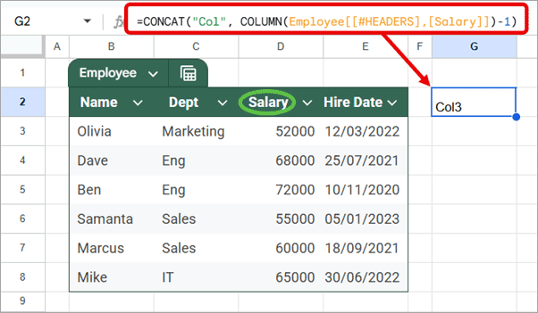
Google Sheets now supports table references. If you are using tables (via Insert → Table or by converting a range into a table), you can dynamically generate QUERY column identifiers using the following pattern:

"&CONCAT("Col", COLUMN(TableName[[#HEADERS],[ColumnName]])-n)&"

This expression is used inside the QUERY string to dynamically build column identifiers.

How Table References Work

TableName → The name of your table
ColumnName → The header (column name)
n → Offset based on the starting column of the table:
- 0 if the table starts in column A
- 1 if it starts in column B
- 2 if it starts in column C, and so on

Using table references with COLUMN function to generate dynamic Col identifiers in Google Sheets QUERY

Note: QUERY still requires ColN identifiers. Table references are used here only to generate those identifiers dynamically.

Example 1: Select Columns

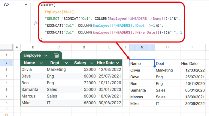
=QUERY(
  Employee[#ALL],
  "SELECT "&CONCAT("Col", COLUMN(Employee[[#HEADERS],[Name]])-1)&", 
  "&CONCAT("Col", COLUMN(Employee[[#HEADERS],[Dept]])-1)&", 
  "&CONCAT("Col", COLUMN(Employee[[#HEADERS],[Hire Date]])-1)&" ", 1
)

This formula selects the Name, Dept, and Hire Date columns.

Google Sheets QUERY using table references to select columns by header names dynamically

Example 2: Group and Aggregate

=QUERY(
  Employee[#ALL],
  "SELECT "&CONCAT("Col", COLUMN(Employee[[#HEADERS],[Dept]])-1)&",
  SUM("&CONCAT("Col", COLUMN(Employee[[#HEADERS],[Salary]])-1)&") WHERE 
  "&CONCAT("Col", COLUMN(Employee[[#HEADERS],[Dept]])-1)&" IS NOT NULL GROUP BY 
  "&CONCAT("Col", COLUMN(Employee[[#HEADERS],[Dept]])-1)&" ", 1
)

This formula groups data by Dept and returns the total Salary for each department.

This method dynamically maps column headers to QUERY-compatible column identifiers using table references, making it resilient to column reordering.

LET vs Table References: Which Should You Use?

Both LET and table references allow you to use column headers dynamically in the QUERY function, but they differ in flexibility and usage:

LET approach
- ✔ Simple to implement
- ✔ No need to convert data into a table
- ✔ Works with any standard range
- ✖ Requires valid variable names (no spaces or special characters)
- ✖ If header names change, you must update them inside the formula
Table references approach
- ✔ Works directly with column headers (no naming restrictions)
- ✔ Automatically adjusts if column headers are renamed
- ✔ More intuitive if you are already using tables
- ✔ Cleaner mapping between headers and columns
- ✖ Requires converting the range into a table
- ✖ Slightly more complex due to COLUMN and offset handling

Which one should you use?

Use LET if you are working with normal ranges and want a quick solution.
Use table references if you are working with structured tables and want a more scalable and flexible approach, especially when headers may change.

Can You Use Column Names in Google Sheets QUERY?

No, QUERY does not natively support column names. It only supports column letters or ColN identifiers. This is why workarounds like LET and table references are required.

Conclusion

In this tutorial, you learned two methods to use column headers in the Google Sheets QUERY function. It may feel a bit confusing at first, but once you get familiar with these approaches, they become much easier to use.

A practical approach is to first write your QUERY using standard column identifiers (such as B, C, or Col1, Col2). Then:

In the LET approach, define the headers using LET and replace the column identifiers in the QUERY with the defined variables.
In the table references approach, directly replace the column identifiers using the structured reference notation.

Both methods help make your formulas more dynamic and resilient to changes in your dataset.