Lookup and Hlookup are the two functions that I am going here to use to Lookup first / last values in a row in Google Sheets. The purpose is to get the corresponding values from the header row.

To Lookup the last value in a row I’ll use the LOOKUP function and to Lookup the first value in a row, the suitable function is HLOOKUP.

I know you are expecting a real-life example before proceeding to the two Lookup formulas. Here you go!

The scenario is like this. I have a header row contain dates in sequential order (date of receipt of payments). Below that, in each row, some of the cells contain values, i.e. payments.

I just want to get the first and last payment receipt dates in each row. The animated screenshot (GIF image) below illustrates it even better.

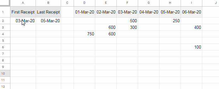
In cell A2 I have an Hlookup formula to Lookup the first value in the row D2:I2, which is 500, and return the corresponding header from D1:I1, which is 03-Mar-20.

Similarly, in cell B2 I have a Lookup formula to Lookup the last value in that row, i.e. 250, and return the corresponding header, i.e. 05-Mar-20.

The Lookup formulas should automatically find the first and last values in the row. Then only it can return the dates from the header. How to do that?

Hlookup Function to Lookup First Value in a Row in Google Sheets

The following Hlookup formula is in the cell A2 in my sheet which copied down.

=ArrayFormula(ifna(hlookup(TRUE,{1/D2:I2<>"";$D$1:$I$1},2,0)))

The above formula is to Lookup the first value in row # 2 and returns the header from row # 1.

Formula Explanation

Here is the Hlookup syntax for your quick reference.

HLOOKUP(search_key, range, index, [is_sorted])

Here are the arguments used as per the formula above.

search_key: TRUE
range: {1/D2:I2<>"";$D$1:$I$1}
index: 2
is_sorted: 0

The Role of IFNA and ARRAYFORMULA in Hlookup

The function IFNA is for removing errors, specifically the #N/A! error, in the output in case the lookup row is blank.

The outer ARRAYFORMULA is for populating a virtual ‘range’. Didn’t get?

In order to get the ‘range’, i.e. {1/D2:I2<>"";$D$1:$I$1}, to work correctly we must use the ARRAYFORMULA function with it. You can use the ARRAYFORMULA with the range only or with the whole formula. I followed the latter.

Now let me explain how the formula helps you Lookup first value (first non-empty cell) in a row and return the header in Google Sheets.

For explanation purposes, I have inserted the below ‘range’ formula in cell D10.

=ArrayFormula({1/D2:I2<>"";$D$1:$I$1})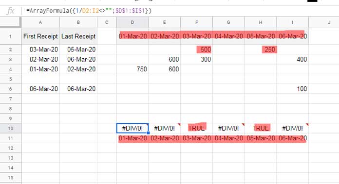

Please check the formula output which is the virtual ‘range’ in Hlookup.

If you check my Hlookup formula, that Lookup the first value in Google Sheets, you can see that the search_key is the Boolean value TRUE. Why it’s so?

As per the above range (D10:I11), or you can say the virtual range, all the non-empty cells corresponding to the row # 2 (D2:I2) contains the Boolean TRUE values.

Now to the logic of the formula.

Hlookup in an unsorted range, see I’ve used is_sorted as 0 in the formula means unsorted, will perform an exact match in the range.

If there are multiple matching values (here multiple TRUE values) in the Hlookup range, the content of the cell (header) corresponding to the first value found is returned.

Lookup Function to Lookup Last Value in a Row in Google Sheets

The following Lookup formula is in the cell B2 which copied down.

=ArrayFormula(ifna(lookup(TRUE,1/D2:I2<>"",$D$1:$I$1)))

The above formula is to Lookup the last value (last non-empty cell) in a row and to return the corresponding value from another row, which is row 1.

Formula Explanation

Here are the Lookup syntaxes:

Syntax 1:

LOOKUP(search_key, search_range, [result_range])

Syntax 2:

LOOKUP(search_key, search_result_array)

In my example, I have used the Hlookup Syntax 1. So based on that, here are the arguments used to Lookup the last value (non-empty cell) in row # 2 and return the header.

search_key: TRUE
search_range: 1/D2:I2<>""
result_range: $D$1:$I$1

The purpose of using IFNA and ARRAYFORMULA is already explained in the first example. The same is applicable here also.

I have keyed the range formula in cell D10 to just to show you the result.

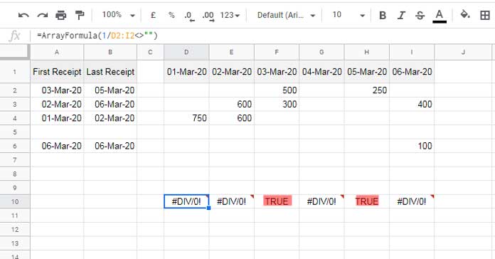
You have seen the use of the search_key, which is Boolean TRUE, in the Hlookup example above.

Now please note that we have used the Lookup Syntax-1 which is called the result_range method. In this method, the result will be from the result_range, i.e. D1:I1.

That means the search_key TRUE matches twice in the ‘range’ and the last column contains the match is in column H. So the corresponding value from the result_range (row 1) returned.

Want the formula as per Syntax 2, i.e. in search_result_array, method?

Simply modify the Hlookup formula as below and use it in cell B2 instead of the above result_range formula.

=ArrayFormula(ifna(lookup(TRUE,{1/D2:I2<>"";$D$1:$I$1})))

That’s all about how to Lookup first and last values (first and last non-empty cells) in a row in Google Sheets.

Related Resources

• Count From First Non-Blank Cell to Last Non-Blank Cell in a Row in Google Sheets.
• Google Sheets: How to Return First Non-blank Value in A Row or Column.
• Find the Cell Address of a Last Used Cell in Google Sheets.
• Find the Last Non-Empty Column in a Row in Google Sheets.
• How to Find the Last Value in Each Row in Google Sheets.
• Vlookup Last Record in Each Group in Google Sheets.
• Lookup to Find the Last Occurrence of Multiple Criteria in Google Sheets.
• Lookup Last Partial Occurrence in a List in Google Sheets.
• Address of the Last Non-Empty Cell Ignoring Blanks in a Column in Excel/Sheets.