With the help of the FILTER function, we can easily create a list from a single column of checked checkboxes in Google Sheets.

But what if there are multiple columns with checkboxes? Instead of copying the formula for each column, we can use BYCOL to apply FILTER across multiple columns in one go.

Introduction to Creating a List from Multiple Column Checkboxes

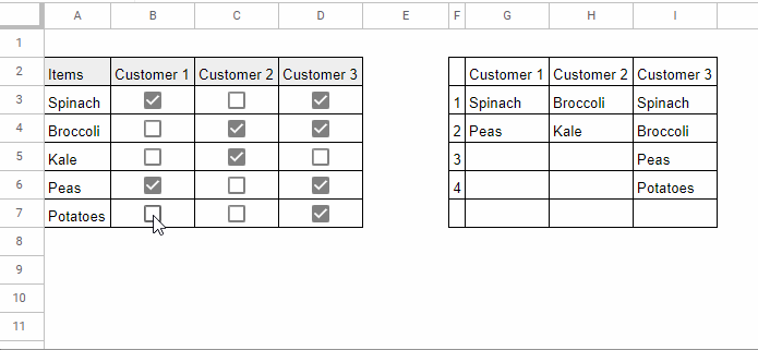
I have a list of vegetables (items) in the first column, and customers’ selections are in the next three columns.

I want to create a customer-wise list of selected items, so that the output shows customer names with their chosen items, instead of just checkboxes.

As mentioned, we can either use a drag-down formula or a dynamic array formula. Both are simple to apply and understand.

1. Create a Non-Dynamic List from Checked Checkboxes

The sample data is in A2:D7. Let’s create the list starting from column F.

In F2, insert the following formula:

=VSTACK(B2, FILTER($A$3:$A$7, B3:B7))

Copy it to G2 and H2.

Here’s how it works:

• The formula filters the vegetables in A3:A7 if the checkbox in B3:B7 is checked.
• The vegetable list range $A$3:$A$7 is absolute, so it won’t change when copied across.
• The checkbox range B3:B7 is relative, so it adjusts automatically for each column.
• VSTACK adds the column header (customer name) on top of the filtered list.

This is the easiest way to create a list from multiple column checkboxes in Google Sheets.

The next method avoids copying formulas across columns.

2. Create a Dynamic List from Multiple Column Checkboxes

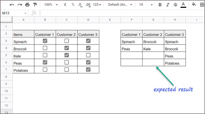
If you want the whole result in one go, use this dynamic array formula in F2:

=VSTACK(B2:D2, BYCOL(B3:D7, LAMBDA(col, FILTER(A3:A7, col))))

This formula generates the complete list in a single step.

How the Formula Works

• FILTER(A3:A7, col) → returns the vegetables where the checkbox is checked.
• BYCOL(B3:D7, …) → applies this logic to each column of checkboxes.
• VSTACK(B2:D2, …) → adds the header row (customer names) above the results.

Additional Tip: Excluding Columns Without Labels

In the above example, we generated a three-column dynamic list.

With the drag-down formula, you can choose which columns to include. But the dynamic array formula doesn’t skip empty headers by default.

This becomes important if you have several checkbox columns, but some don’t have labels. For example, if you remove the label "Customer 2", you probably don’t want that column in the output.

To omit unlabeled columns, use this adjusted formula:

=VSTACK(
  FILTER(B2:D2, B2:D2<>""), 
  BYCOL(FILTER(B3:D7, B2:D2<>""), LAMBDA(col, FILTER(A3:A7, col)))
)

This version filters both the headers and the corresponding checkbox columns, removing any without labels.

Example Sheet

Resources

• Inserting Check Marks and Checkboxes in Google Sheets
• Assign Values to Checkboxes and Calculate Totals in Google Sheets
• Change Checkbox Color While Toggling in Google Sheets
• 10 Best Checkbox Tips and Tricks in Google Sheets
• Check/Uncheck a Checkbox Based on Another Cell in Google Sheets
• Convert TRUE or FALSE to Checkboxes in Google Sheets
• Lock and Unlock Cells Using Checkboxes in Google Sheets
• Highlight Multiple Groups Using Checkboxes in Google Sheets
• VLOOKUP in Checkbox Checked Rows in Google Sheets