TRUE and FALSE are Boolean values. You can convert these values to checkboxes since checkboxes itself returns TRUE (checked) or FALSE (unchecked). It’s possible to convert TRUE/FALSE to checkboxes in Google Sheets.
You may have the Boolean TRUE/FALSE in a cell or column as an output of any formula or manually entered as a text string. In both the cases, you can convert the TRUE/FALSE values to checkboxes.
I have already detailed the use of dependent tick boxes in Google Sheets. Tick boxes are another name of checkboxes. This tutorial is in line with that earlier tick box tutorial.
Note: You can insert tickboxes in Google Sheets from the Insert Menu.
Let’s see how to format or convert TRUE/FALSE to tick boxes/checkboxes.
Convert TRUE/FALSE to Checkboxes in Google Sheets
Scenario 1:
Convert Existing Manually Entered TRUE/FALSE to Checkboxes
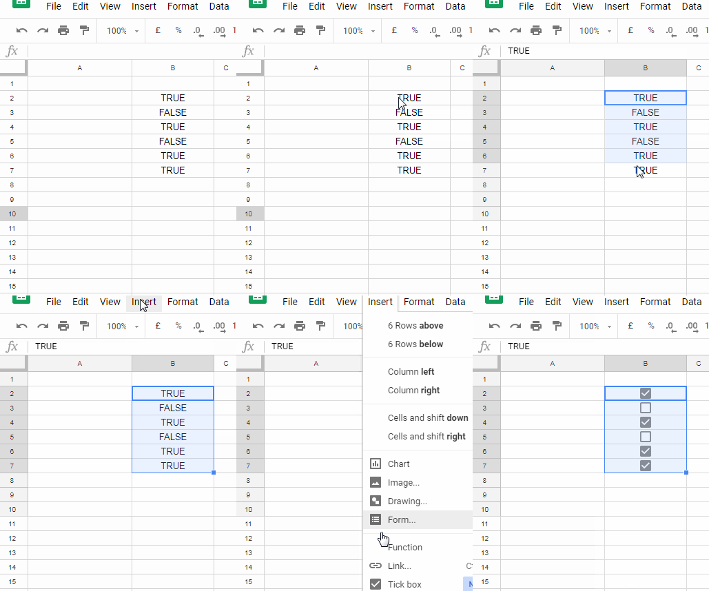
It’s very easy and quick to convert a column with the Boolean TRUE/FALSE to tick boxes in Google Sheets. You just need to select the cells and then go to the menu Insert and click on Tick Box.

Scenario 2:
Convert Boolean TRUE/FALSE Formula Outputs to Checkboxes
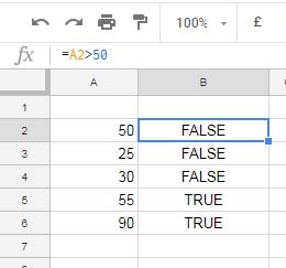
Here you can follow two methods. As an example let me show you a simple logical test using a comparison operator which returns the Boolean TRUE/FALSE.
Must Read: IF, AND, OR Logical Test in Google Sheets.

The formula in cell B2 copied down. How to convert these TRUE/FALSE values to checkboxes in Google Sheets.
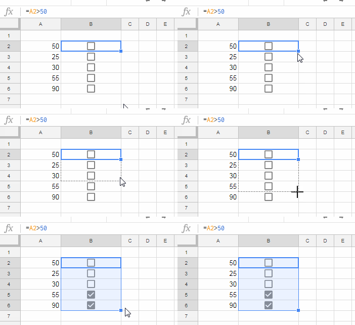
No doubt. Just select the cells in the range B2:B6 and then go to the Insert menu and select Tick Box.
There is one more method. First, insert the tick boxes and then apply the formula.

That’s it. To convert TRUE/FALSE to Checkboxes in Google Sheets follow the above simple steps.
Advanced users can even use this feature to Match two columns for duplicates and then tick mark the duplicates. You can follow the below method to dynamically convert TRUE/FALSE to Checkboxes in Google Sheets.
Scenario 3:
Match Two Columns and Convert TRUE/FALSE to Checkboxes in Google Sheets
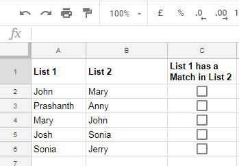
Here is a simple example in this I’ll show you how to compare two columns and convert Match/Mismatch to Checkboxes in Google Sheets.
You May Like: Google Sheets: How to Compare Two Tables and Remove Duplicates.
In the below example I am going to check the availability of the names in Column A in Column B. If found I want to check and uncheck the checkboxes accordingly.
Steps:
1. Insert Checkboxes in C2:C6.

2. Use the below formula in cell C2 and drag down.
=IFERROR(if(match(A2,$B$2:$B,0)>0,TRUE),FALSE)
That’s all. Enjoy!
Additional Resources:
1. Assign Values to Tick Box and Total It in Google Sheets.
2. Change the Tick Box Color While Toggling in Google Sheets.
3. 10 Best Tick Box Tips and Tricks in Google Sheets.
4. Remove Duplicates in Google Sheets [The Complete Guide and Sample Sheet].


