The ISLOGICAL function in Google Sheets is an info-type function. That means you can use it to gather information about a value in a cell.

The ISLOGICAL function is useful for identifying Boolean values in Google Sheets.

What Are Boolean Values?

Boolean values are logical values—TRUE or FALSE—commonly used in formulas to represent conditions like yes/no or on/off. In Google Sheets, these values are also treated as numbers:

• TRUE is equivalent to 1
• FALSE is equivalent to 0

You can manually type them, generate them with logical functions like AND or OR, or use checkboxes to input them visually.

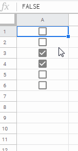
Tick Boxes in Google Sheets Place Boolean Values in Cells

Tick boxes in Google Sheets typically store Boolean values—TRUE when checked and FALSE when unchecked—unless customized to return other values.

Logical Formulas That Return Boolean Values

Here is an example using the AND function, which returns either TRUE or FALSE:

=AND(A2>0, B2<5)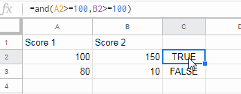

Other logical functions—like IF, OR, and XOR—can also return Boolean values. You can find these under the “Logical” category in my Functions Guide.

Simply typing TRUE or FALSE into a cell will also be treated as a Boolean input in Google Sheets.

Now, let’s return to the ISLOGICAL function.

Purpose of ISLOGICAL in Google Sheets

The sole purpose of ISLOGICAL is to check whether a given value is a Boolean—i.e., TRUE or FALSE.

Example: Using ISLOGICAL in Google Sheets

In the following example, the ISLOGICAL formula tests the value in cell C2:

=ISLOGICAL(C2)

This function tests for the presence of Boolean values and returns a Boolean output.

To convert that output into a number (1 for TRUE, 0 for FALSE), use the double unary operator:

=--ISLOGICAL(C2)

ISLOGICAL with ArrayFormula

The ISLOGICAL function also works well with arrays. To test a range of values (e.g., C2:C12), use:

=ArrayFormula(ISLOGICAL(C2:C12))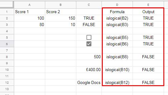

Practical Use Cases of ISLOGICAL in Google Sheets

It’s important to know where ISLOGICAL can be applied in real-world scenarios. Here are three different use cases:

1. As a worksheet formula
2. As a custom formula in Conditional Formatting
3. In data validation

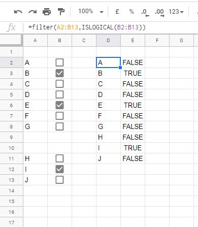
Example: ISLOGICAL with FILTER Function

Problem: Filter rows where column B contains a checkbox.

=FILTER(A2:B13, ISLOGICAL(B2:B13))

This formula filters only the rows where column B contains Boolean values (checkboxes).

Highlight Boolean Values Using ISLOGICAL in Google Sheets

Use Conditional Formatting to highlight cells containing TRUE, FALSE, or checkboxes.

Steps:

1. Select the range A1:E13
2. Go to Format > Conditional formatting
3. Under “Format rules,” choose Custom formula is
4. Enter this formula:=ISLOGICAL(A1)

This will apply formatting to all cells in the selected range that contain Boolean values.

Using ISLOGICAL in Data Validation to Restrict Inputs to Boolean Values

You can use the ISLOGICAL function in data validation to ensure that only Boolean values (TRUE or FALSE) or checkboxes are accepted in a cell or range.

Steps:

1. Select the range where you want to restrict input (e.g., B2:B10).
2. Go to Data > Data validation.
3. Under Criteria, choose Custom formula is.
4. Enter the formula:
   =ISLOGICAL(B2)
5. Choose to Reject input if the condition is not met.
6. Click Done.

Now, only cells containing Boolean values, formulas that return TRUE or FALSE, or checkboxes will be accepted, preventing manual entry of non-Boolean text or numbers.

Additional Reading:

• Convert TRUE or FALSE to Checkboxes in Google Sheets
• The Role of the TRUE Logical Function in Google Sheets
• Google Sheets FALSE Function – How to and Examples
• 10 Best Tick Box Tips and Tricks in Google Sheets
• Return a Value When Expression is FALSE in IFS in Google Sheets