TRUE is a Boolean value representing one of the two truth values in logic. The other truth value, also known as a logical value, is FALSE. You can obtain the TRUE Boolean value by using the TRUE logical function in Google Sheets.

Instead of using the TRUE() function, you can enter TRUE directly in most cases in Google Sheets. It will interpret such input values as Boolean values.

You can add, subtract, and divide Boolean values because TRUE has a numeric value of 1 and FALSE has a numeric value of 0.

Example Formula:

=TRUE()+TRUE()

Result: 2

Here are a few ways to input or generate the Boolean value TRUE in Google Sheets:

1. Using an Expression

• Enter a value like 10 in cell A1.
• In another cell, use the formula =A1=10 or =EQ(A1, 10). This will return TRUE because the value in A1 is indeed equal to 10.

2. Entering the Text “TRUE”

• Simply type TRUE (case insensitive) in any cell. Google Sheets will automatically recognize it as the Boolean value TRUE.
• To test this, enter TRUE in cell A1. In cell B1, use the formula =A1+1. It will return 2 because TRUE is treated as the number 1 for calculations.

3. Using the =TRUE() Function

• Enter the formula =TRUE() in any cell. This explicitly returns the Boolean value TRUE.

How to Use the TRUE Function in Google Sheets

Syntax:

TRUE()

Boolean values are fundamental for conditional statements in spreadsheets. This means you can use the TRUE function along with other logical functions like IF, AND, and OR to create complex conditions.

TRUE with IF Function

To check if a student’s mark in cell B2 is above 50, you can use the IF function in cell C2. Here are two options for the formula:

=IF(B2>50, TRUE)
=IF(B2>50, TRUE())

This IF formula evaluates the condition B2>50. If the mark in B2 is greater than 50, the formula returns TRUE.

Since the IF function only specifies a value to return if the condition is true, it inherently returns FALSE if the condition is not met (i.e., the mark is less than or equal to 50). There’s no need to explicitly specify FALSE.

If you prefer to “mute” the FALSE output, you have two options:

1. Leaving the Second Argument Empty:

This is shown in the formulas:

• =IF(B2>50, TRUE, )
• =IF(B2>50, TRUE(), )

An empty second argument instructs the IF statement to return nothing for the FALSE condition, effectively muting it.

2. Using an Empty String (“”) for FALSE:

You can also use an empty string to represent a “muted” FALSE output:

• =IF(B2>50, TRUE, "")
• =IF(B2>50, TRUE(), "")

While muting the FALSE output might seem visually appealing, it’s generally recommended to explicitly return a value (like FALSE or 0) for the FALSE condition to ensure clarity in your data.

TRUE with AND and OR in IF Statements

We can use the IF function along with AND and OR operators to create more complex conditions for returning TRUE or FALSE.

Related: Combined Use of IF, AND, and OR Logical Functions in Google Sheets

The following formula tests whether the marks in B2, C2, and D2 are greater than 50. If all conditions are met, the formula will return TRUE; otherwise, it will return an empty string:

=IF(AND(B2>50, C2>50, D2>50), TRUE(), "")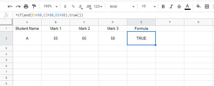

Alternative Formula:

=IF(AND(B2>50, C2>50, D2>50), TRUE, "")

Similarly, you can use the IF function to check if any mark in cells B2, C2, or D2 is greater than 50. Here are two functionally equivalent formulas:

=IF(OR(B2>50, C2>50, D2>50), TRUE, "")
=IF(OR(B2>50, C2>50, D2>50), TRUE(), "")

Logical Function TRUE in Inserting Non-Toggleable Tick Boxes

If you enter TRUE in a cell and click Insert > Tickbox, you will get a checked tickbox. You can toggle the tickbox without any issue, as it will convert the underlying value to TRUE or FALSE.

However, if you want to insert a checked tickbox that cannot be toggled to FALSE, enter =TRUE() in a cell and click Insert > Tickbox.

Example:

Query WHERE Clause and Boolean Values

In my tutorial on using literals in QUERY, you can see how to use the TRUE boolean literal.

The correct way to use the Boolean literal TRUE in a Query WHERE clause is as follows:

=QUERY(A2:B, "SELECT * WHERE B=TRUE")

You should not use TRUE() instead of TRUE in the QUERY formula because TRUE() is a function that evaluates to TRUE.

Resources

• How to Return Value When The Logical Expression is FALSE in IFS
• Using OR Logical Function to Return Expanded Results in Google Sheets
• How to Use AND Logical in Array in Google Sheets
• How to Use Percentage Value in Logical IF in Google Sheets
• How to Use Timestamp within IF Logical Function in Google Sheets
• Logical AND, OR Use in SEARCH Function in Google Sheets
• Defining Explicit Precedence in Google Sheets Query (Logical Operators)
• How to Use AND and OR with the Google Sheets FILTER Function