Google Sheets FALSE function returns the FALSE Boolean value. Without using this logical function, you can get the Boolean value FALSE in a few other ways in Docs Sheets.

Entering the text value FALSE in a cell or formulas will be converted to the Boolean value FALSE in most of the cases in Google Sheets.

If you want the FALSE value in a cell, you can follow any of the below methods.

1. Simply type FALSE (case insensitive) in a cell.
2. =FALSE
3. FALSE()

Note: Wherever you see FALSE in this post, read it as Boolean FALSE.

To refer to the value FALSE in formulas you can use either of method 1 or 3. But in Query, the 1st method will only work.

Syntax of the FALSE Logical Function:

See the Syntax below. There is no argument to use in this logical function.

FALSE()

How to Use the FALSE Function in Google Sheets

Example 1: Return FALSE if the logical expression evaluates false.

=A1=20

This formula will return TRUE if the value in cell A1 is 20, else it will return FALSE. Here is the equivalent logical test.

=if(A1=20,TRUE,FALSE)

Here you can replace TRUE with the TURE() function and FALSE with the FALSE() function as below.

=if(A1=20,TRUE(),FALSE())

Filter Rows If Values in a Column Are Boolean Types

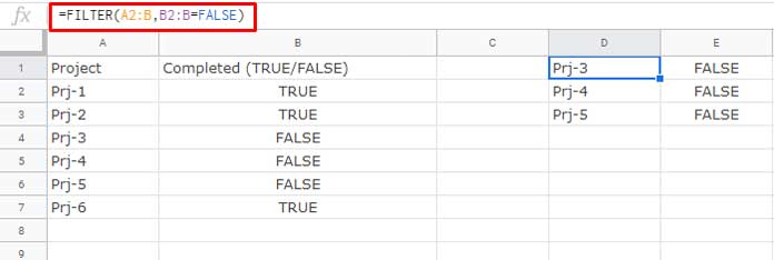
This example is to show you how to use the FALSE function for filtering datasets.

=FILTER(A2:B,B2:B=FALSE)

Here you can replace the criteria with the FALSE() function as below.

=FILTER(A2:B,B2:B=FALSE())

Both the formulas will return the same output. But in Query, you can’t use the FALSE() function. Instead, simply use the text FALSE.

=query(A2:B,"Select A,B where B=FALSE")

If you use text criteria in Query, it should be within single or double-quotes. Here note, I didn’t include the criteria within quotes.

Additional Tips

To convert FALSE to 0 and TRUE to 1, wrap the formula with the N function.

For example cell A1 contains FALSE. Use this formula.

=N(A1)

Another tip is formatting the FALSE value in Google Sheets. Select the cells that contain the FALSE value. Go to Insert > Tick box. The value will be converted to an unchecked tick box that you can toggle.

If the cell contains a FALSE() function, then that value can also be formatted as above. The difference here is you can’t check or uncheck the tick box.