The ISFORMULA function in Google Sheets is one of the useful tools for ensuring that your spreadsheet is set up correctly.
It can identify cells with formulas by employing it in conditional formatting or testing each cell individually.
The ISFORMULA function is not an array function. When applied within a cell, it can check only one cell at a time. However, when used in conditional formatting for a range, it can test each cell and highlight those with formulas.
Recent developments in Google Sheets have made ISFORMULA even more useful. With the introduction of Lambda helper functions, you can now use the ISFORMULA function in each cell in a range.
For example, you can test the range A1:A100 and count how many cells contain formulas.
Syntax:
ISFORMULA(cell)Where ‘cell’ is the cell to check for a formula.
Examples
In the following example, the value in cell A2 is 10, cell B2 is 2, and the formula in cell C2 is =A2*B2.
You will see the result 20 in cell C2. If you navigate to cell C2, you can see the formula in the formula bar.
If you need to test whether cell C2 contains a formula and return the Boolean value TRUE or FALSE, you can use the following ISFORMULA formula in cell D2:
=ISFORMULA(C2)This will return TRUE because there is a formula in cell C2. If you remove the formula, it will return FALSE.
As a side note, if you want to see the formula in cell C2 displayed in cell D2 instead, you can use the FORMULATEXT function as follows:
=FORMULATEXT(C2)Using the ISFORMULA Function in Logical Tests in Google Sheets
Since the ISFORMULA function in Google Sheets returns a Boolean value, you can use it within logical tests.
For example, you can check whether a cell contains a formula and return custom text instead of TRUE or FALSE.
The following formula will return a tick mark if cell C2 contains a formula, or a cross mark if it does not:
=IF(ISFORMULA(C2), "✔", "X")This formula will return a blank for a formula and the text “Warning!” if there is no formula:
=IF(ISFORMULA(C2), "", "Warning!")Counting Formulas in a Range Using COUNTIF with ISFORMULA and the MAP Lambda Function
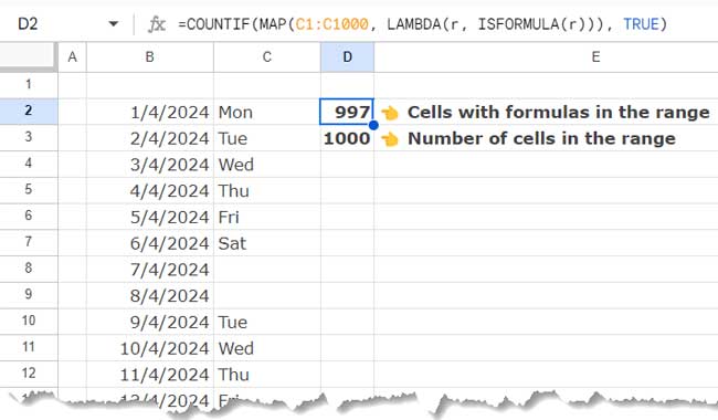
Here is how to use the ISFORMULA function in a range of cells in Google Sheets.
Assuming you have non-array formulas in cells C1:C1000, you want to check if all the formulas are still intact or if any have been accidentally replaced with some real values.
You can use the following formulas:
The following formula will return the number of cells containing formulas:
=COUNTIF(MAP(C1:C1000, LAMBDA(r, ISFORMULA(r))), TRUE)And this one will return the total number of cells in the range:
=ROWS(C1:C1000)
If the numbers are different, it indicates there is an issue.
You can easily highlight the formula cells using an ISFORMULA-based highlight rule. Please check out my tutorial on that: How to Highlight All the Cells with Formulas in Google Sheets.
Formula Breakdown
The MAP function maps each value in the array C1:C1000 and returns new values by applying a lambda. The lambda here is LAMBDA(r, ISFORMULA(r)), where r represents the current element in the array.
The COUNTIF function returns the count of cells that meet a specified condition. In this case, it counts the cells where the ISFORMULA function evaluates to TRUE.
Resources
- How to Use ISREF Function in Google Sheets [Formula and Examples]
- How to Use ISTEXT Function in Google Sheets [Example Formulas]
- How to Use the ISERROR Function in Google Sheets
- Difference Between ISERR and ISNA Functions in Google Sheets
- Practical Use of ISBLANK Function in Google Sheets
- How to Use ISNONTEXT Function in Google Sheets [Practical Use]
- How to Use ISEVEN Function in Google Sheets [Formula Examples]
- ISDATE Function and Better Alternative in Google Sheets
- How to Use the ISLOGICAL Function in Google Sheets
- Google Sheets ISODD Function – Formula Examples
- The ISURL Function in Google Sheets – Check/Highlight/Validate URLs
- How to Use the ISBETWEEN Function in Google Sheets


