The INT function in Google Sheets rounds a number down to the nearest integer if the original number contains a fractional part; otherwise, it returns the same number.
To better understand the function, we will apply it with both positive and negative numbers.
This tutorial describes how to use the INT function in both array and non-array forms in Google Sheets. Before we delve into that, here is the function syntax.
Syntax of the INT Function in Google Sheets
Syntax:
INT(value)
Arguments:
value: The number to round down if it has a fractional part; otherwise, retain the same.
The value can be a number entered within the formula (hardcoded) or a cell reference. If you refer to an array or range as the value argument, include the ArrayFormula. Additionally, you may want to include the IFERROR function as part of the formula to handle errors and an IF logical test to exclude zeros. We will explore these aspects in the examples below.
Examples of the INT Function
In the first two examples, I am hardcoding the ‘value’ within the formula.
=INT(600.25) // returns 600The above formula will return 600. However, if the value is -600.25, the result would be -601.
=INT(-600.25) // returns -601If the number is 600 or -600, the output will be the same number.
In summary, for positive numbers, the INT function in Google Sheets rounds down towards 0, and for negative numbers, it rounds towards negative infinity.
Note: In all the above examples, you can enter the value in a cell, for example, cell A1, and enter the formula as follows:
=INT(A1)In the following table, the first column contains the values, and the second column contains the output returned by INT.
| Value | Output |
| 12.95 | 12 |
| -12.95 | -13 |
| 10 | 10 |
| -10 | -10 |
| 0 | 0 |
How to Round Down Values in a Range to the Nearest Integer
We have already discussed the array formula capability of the INT function. When you use it with an array, employ the ARRAYFORMULA function.
Example:
=ArrayFormula(INT(A2:A11))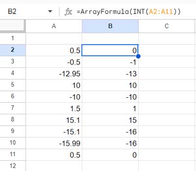
If you want to use the INT function to round down values to the nearest integer and sort, then replace ARRAYFORMULA with SORT.
=SORT(INT(A2:A11))Furthermore, you can round down to the nearest integer and get the max or min n values using SORTN.
Max 3:
=SORTN(INT(A2:A11), 3, 0, 1, 0)Min 3:
=SORTN(INT(A2:A11), 3)Utilizing the INT Function in an Open Range in Google Sheets
In the above INT function array formula examples, the range in use is closed. If it’s open, you may get unexpected results while sorting.
This is because the INT function will return 0 when referring to a blank cell as the value.
How do we correctly use the INT function in an open range?
We need to employ an IF logical test that involves the IF and ISNUMBER functions. Here is an example:
=ArrayFormula(IF(ISNUMBER(A2:A), INT(A2:A),))This is the proper way to use the INT function in an open range in Google Sheets. In this, you can replace ARRAYFORMULA with SORT or SORTN as needed.
Conclusion
In this tutorial, we explored how to use the INT function in both array and non-array forms in Google Sheets.
Regarding errors, the INT function returns a #VALUE error when the value is text. This can be managed by using the IF and ISNUMBER combination, as demonstrated with open ranges.
For instance, if the value is in cell A1, you can use this formula:
=IF(ISNUMBER(A1), INT(A1), )Alternatively, you can wrap the INT formula with IFERROR as follows:
=IFERROR(INT(A1))However, when dealing with open ranges, I highly recommend using the IF and ISNUMBER combination to address blank cells in the range.
Instead of rounding down, if you simply want the whole number part of a value without any rounding behavior, use the TRUNC function.
Unlike INT, which rounds toward zero for positive numbers and negative infinity for negative numbers, TRUNC completely discards the decimal part, leaving you with the integer portion.


