Date difference as criteria refers to the duration between dates or dates falling between two given dates. In this Google Sheets tutorial, I will guide you on how to utilize date differences as criteria in the SUMPRODUCT function.

Assume you want to use SUMPRODUCT for conditional sum (using a date criteria column and an amount column). What about functions like SUMIFS and DSUM (conditional sum functions) with the same type of criteria?

The usage of date criteria in DSUM is almost identical to the usage of date criteria in SUMIFS. If you are new to this as well, I have already provided detailed tutorials.

• DSUM: How to Use Date Difference As Criteria in DSUM in Google Sheets
• SUMIFS: How to Include a Date Range in SUMIFS in Google Sheets

However, the usage of date criteria in SUMPRODUCT is slightly different. I will explain it below with an example.

The date field as a criterion in the SUMPRODUCT function is one of the areas where you should pay attention. When dealing with multiple criteria in SUMPRODUCT, you may falter otherwise.

Using Date Differences as Criteria in SUMPRODUCT in Google Sheets

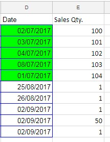
In this illustration, I am summing the “Sales Qty.” for sales that occurred between 01/07/2017 and 31/07/2017.

Observe how SUMPRODUCT is used with date criteria in Google Sheets.

Here is the formula for this somewhat uncommon SUMPRODUCT date criteria. Typically, Google Sheets users prefer SUMIFS or DSUM in such scenarios.

=SUMPRODUCT((D2:D11>=DATE(2017, 7, 1))*(D2:D11<=DATE(2017, 7, 31))*(E2:E11))

Note: In the formula, we have specified the date using the syntax DATE(year, month, day)

In addition to the date criteria in SUMPRODUCT, there’s another noteworthy element in this formula—the use of multiple criteria in the same field. Pay attention to the brackets used in the formula.

In the above formula that employs date difference as criteria in SUMPRODUCT, I’ve utilized the same “Date” field, i.e., D2:D11, twice.

With the above example, you can grasp the following points:

When using multiple criteria in the same field, employ the formula as follows (only the date part is shown):

(D2:D11>=DATE(2017, 7, 1))*(D2:D11<=DATE(2017, 7, 31))

When using a single criterion in the same field, use the formula as follows:

D2:D11=DATE(2017, 7, 1)

These formulas (criteria test) return an array of values with 1 (TRUE) or 0 (FALSE). Multiplying them with the ‘Qty’ column and summing them equals the total quantity, and that is what the SUMPRODUCT does.

Conclusion

I hope you found answers to the following queries in the tutorial:

• How to use date differences as criteria in SUMPRODUCT in Google Sheets?
• How to use multiple criteria in the same field or array in Google Sheets?
• Finally, how to use multiple criteria in SUMPRODUCT?

The SUMPRODUCT function is easy to learn and use. Many people encounter errors when using functions like SUMPRODUCT, SUMIFS, or DSUM due to variations in criteria.

To overcome this, my suggestion is to stick with the function that suits you best and is easy to learn.

Resources:

• Difference Between SUMIFS and SUMPRODUCT in Google Sheets
• Compare Sumifs, Sumproduct, and Dsum with Examples in Google Sheets
• Chart to Learn Text, Date, Numeric Criteria in Sumproduct Function in Google Sheets
• How to Do a Case Sensitive Sumproduct in Google Sheets
• How to Use OR Condition in SUMPRODUCT in Google Sheets
• How to Use Wildcards in Sumproduct in Google Sheets
• How to Use Sumproduct with Merged Cells In Google Sheets