Why is it important to learn how to correctly specify criteria in the SUMPRODUCT function, given its role in calculating the sum of products?
SUMPRODUCT is an array function in Google Sheets used for finding the sum or products. Additionally, it can be employed for conditional sums or counts, depending on the criteria applied. Therefore, it’s crucial to understand the proper specification of text, date, and numeric criteria with this function.
You must know how to hardcode as well as use cell references when specifying criteria in functions, as it might slightly vary from function to function.
Allow me to assist you in mastering the specification of text, date, and numeric criteria within the SUMPRODUCT function in Google Sheets. Below, you’ll find a simple chart (table) that will aid in this process.
We will use the following sample data for reference:
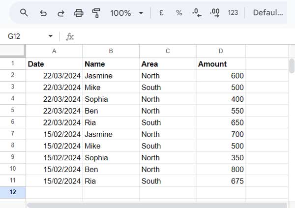
In the sample data, column A contains the sales date, Column B contains the name of the salesperson, Column C contains the area of sales, and Column D contains the sales amount. The actual data range is not A1:D, but A1:D11, where A1:D1 contains field labels.
Sumproduct Criteria Specification Reference Chart
In the table below, the first column describes the type of criteria you want to use, the second column demonstrates how to specify hard-coded criteria, and the third column indicates what you should enter in cell F1 to specify it in the formula.
| Data Type | Hardcoded | Cell Reference (F1) | Example Formula |
| Text: | |||
| “North” | North | =SUMPRODUCT(=SUMPRODUCT( | |
| Numeric: | |||
| 500 | 500 | =SUMPRODUCT(=SUMPRODUCT( | |
| >500 | 500 | =SUMPRODUCT(=SUMPRODUCT( | |
| Date: | |||
| DATE(2024, 3, 22) | 22/03/2024 DD/MM/YYYY or MM/DD/YYYY | =SUMPRODUCT(=SUMPRODUCT( | |
| >DATE(2024, 3, 20) As per: DATE(year, month, day) | 20/03/2024 DD/MM/YYYY or MM/DD/YYYY | =SUMPRODUCT(=SUMPRODUCT( |
Specifying Multiple Criteria
In all the above examples, we have used a single criterion. You can follow the same syntax when specifying multiple criteria in the SUMPRODUCT function.
For example, assume you want to count the number of sales in the “South” region in March 2024. You can use the following SUMPRODUCT for that:
=SUMPRODUCT(
   (C2:C11="South")*
   ((EOMONTH(A2:A11, -1)+1)=DATE(2024, 3, 1))
)
In this formula, the EOMONTH function returns the end of the month dates of the dates in the range A2:A11. Adding 1 to that converts it to the beginning of the month dates. So we can use 01/03/2024 as the criterion.
In this complex SUMPRODUCT formula, we have specified hard-coded criteria. How do we specify criteria as cell references?
=SUMPRODUCT(
   (C2:C11=F1)*
   ((EOMONTH(A2:A11, -1)+1)=F2)
)
Specify “South” (without double quotes) in cell F1 and 01/03/2024 in cell F2.
If your sales data in A2:A11 are contained within 2024, you do not need to worry about using the EOMONTH function. You can simply specify the month number in the formula as follows:
=SUMPRODUCT(
   (C2:C11="South")*
   ((MONTH(A2:A11)=3)
)
The EOMONTH approach is particularly useful in formulas when you want to consider both the month and year instead of just the month. If you do not use EOMONTH, then you might want to use two criteria, one for matching the month and the other for matching the year.
Resources
You now have a chart to refer to on how to correctly specify criteria in the SUMPRODUCT function in Google Sheets. Additionally, I’ve provided a couple of examples that clearly demonstrate the use of criteria. Here are some additional resources.
- How to Use Date Differences as Criteria in SUMPRODUCT in Google Sheets
- Differences Between SUMIFS and SUMPRODUCT Functions in Google Sheets
- Comparing SUMIFS, SUMPRODUCT, and DSUM with Examples in Google Sheets
- How to Do a Case Sensitive Sumproduct in Google Sheets
- How to Use OR Condition in SUMPRODUCT in Google Sheets
- How to Use Wildcards in Sumproduct in Google Sheets
- How to Use Sumproduct with Merged Cells In Google Sheets


