


")


")

")
")
 in Excel & Google Sheets")


The HYPERLINK function in Google Sheets allows you to label URLs, making them more user-friendly by displaying custom text instead of the full web address. In this post, we’ll explore how to label a URL in Google Sheets using the HYPERLINK function.
What Is a URL?
A URL (Uniform Resource Locator) is simply the web address of a website or a webpage. When you open a webpage in your browser, you can find the URL in the address bar at the top.
As a side note, in a Google Sheets file (workbook) with multiple sheets, each sheet has its own specific URL, and you can even generate a URL for individual cells. To get a cell’s URL, right-click on the cell, then in the menu that appears, click View more cell actions > Get link to this cell. This allows you to easily share or reference specific cells within a Google Sheets document.
What Does “Labeling a URL” Mean?
Labeling a URL refers to replacing a long, cumbersome web address with a short, readable label or title that represents the link. Instead of displaying a URL like https://example.com/, you can use the HYPERLINK function to display it as “Click Here” or any other custom text. This makes spreadsheets cleaner and easier to read.
Example of Labeling a URL in Google Sheets
Take a look at the following example:
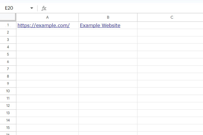
- In cell A1, you see a raw URL:
https://example.com/ - In cell B1, you see a labeled URL:
Example Website
Both are clickable and clicking either will take you to the same webpage. The difference is that the labeled link in B1 is much cleaner and more readable.
Labeling URLs Using the HYPERLINK Function
To label a URL in Google Sheets, you use the HYPERLINK function. Here’s the syntax:
Syntax:
HYPERLINK(url, [link_label])- url: The web address (URL) you want to link to.
- link_label: The text you want to display for the link (optional). If you omit this, the URL itself will be displayed.
Example:
=HYPERLINK("https://infoinspired.com/google-docs/spreadsheet/google-sheets-function-guide/", "Function Guide")In this example, the URL points to a webpage, but the link will display as “Function Guide” in the cell, creating a labeled URL.
Important Details When Using HYPERLINK
When using the HYPERLINK function, you need to ensure the URL is correctly formatted. If the protocol (e.g., http:// or https://) is missing, Google Sheets will automatically prepend http://, which might not always be correct. For instance, omitting the protocol can cause issues if you’re working with secure (https://) or specific (ftp://, mailto:) links.
For example, using a URL without the protocol:
=HYPERLINK("example.com", "Example Website")Would result in an incorrect link (http://example.com), potentially causing navigation errors. Always include the full protocol in your URL:
=HYPERLINK("https://example.com", "Example Website")According to official documentation, the supported link types include:
http://https://mailto:aim:ftp://gopher://telnet://news://
Labeling Multiple URLs at Once
If you need to label multiple URLs at the same time, you can use the ARRAYFORMULA function in combination with HYPERLINK. This allows you to apply the HYPERLINK function to a range of URLs, saving you time from manually labeling each one.
Here’s an example of labeling URLs in column A using labels from column B:
=ArrayFormula(HYPERLINK(A2:A6, B2:B6))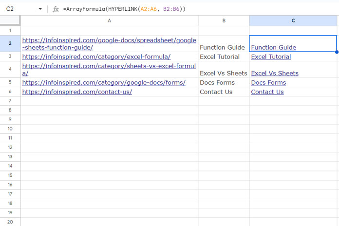
In this example:
- Column A contains the URLs.
- Column B contains the corresponding labels.
- The formula labels all the URLs in A2:A6 using the labels in B2:B6.
This method allows you to easily modify the labels if needed, as you can simply change the text in column B, and the HYPERLINK function will update accordingly.
Conclusion
Now that you know how to use the HYPERLINK function, labeling URLs in Google Sheets becomes much easier. You can create cleaner, more professional-looking spreadsheets by turning long URLs into readable, clickable text.
If you need to label multiple URLs at once, combining HYPERLINK with ARRAYFORMULA can streamline the process and save time. Try it out in your own Google Sheets and enjoy the improved readability!
Resources
- Search Value and Hyperlink Cell Found in Google Sheets
- Create a Hyperlink to the Vlookup Output Cell in Google Sheets
- Extract URLs from Hyperlinks in Google Sheets (No Scripting)
- UNIQUE Duplicate Hyperlinks in Google Sheets – Same Labels Different URLs
- How to Create a Hyperlink to an Email Address in Google Sheets
- Hyperlink Max and Min Values in Column or Row in Google Sheets
- Hyperlink to Index-Match Output in Google Sheets
- Inserting Multiple Hyperlinks within a Cell in Google Sheets
- Hyperlink to Jump to Current Date Cell in Google Sheets
- Jump to the Last Cell with Data in a Column in Google Sheets (Hyperlink)
- Hyperlink Calendar Dates to Events in Google Sheets
- Using HYPERLINK with FILTER Function in Google Sheets