In this tutorial, let’s explore the usage of the BYROW function in Google Sheets, serving as a Lambda Helper Function (LHF). Once you’ve mastered the LAMBDA function, incorporating the BYROW helper function will be a breeze.

How does this LHF prove useful? It introduces new capabilities to Google Sheets. Previously, there were virtually no methods to exclude hidden rows (or include visible rows) in formulas without resorting to a helper column. Now, thanks to the introduction of this function, it’s possible, and I’ll delve into the details later in this tutorial.

For your reference, I’ve provided an example here – “SUMIF Excluding Hidden Rows in Google Sheets [Without Helper Column].” This is achievable because the BYROW function can expand the results of non-expanding formulas such as SUM, MIN, MAX, AVERAGE, SPARKLINE, SUBTOTAL, etc.

Before, we used functions like MMULT, database functions, or QUERY to expand such formula results (not all). Here’s an example where an MMULT replaces SUM:

The MMULT formula in cell F3 can replace the =SUM(B3:D3), =SUM(B4:D4), and =SUM(B5:D5) formulas in F3, F4, and F5.

=MMULT(B3:D5, {1; 1; 1})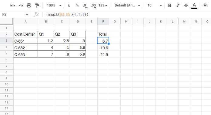

As an alternative, the BYROW function can be used in this context.

Syntax and Arguments

Syntax:

BYROW(array_or_range, lambda)

Arguments:

• array_or_range: The array or range to use in a lambda function by row (e.g., B3:D5 [as per the screenshot above]).
• lambda: A lambda for a single row (e.g., B3:D3 [as per the screenshot above]), usually the first row, to calculate a single result. The BYROW function will expand it in the given array_or_range. It’s important to note that a defined name will be used to represent each element in the array, not B3:D3.

Syntax for LAMBDA:

=LAMBDA(name, formula_expression)(function_call)

Important:

The LAMBDA function can take more than one name argument and function_call, but when used with BYROW, only one name argument should be used, and the function_call should be omitted.

How to Use the BYROW Function in Google Sheets

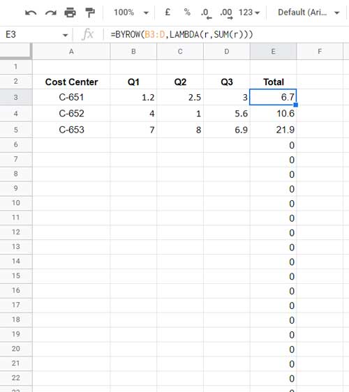
Please scroll up and refer to the image.

In the image, we have an MMULT function used to calculate the total of each row.

To replace it, you can use the following BYROW formula. Clear cells F3:F5 and enter the following code in cell F3.

=BYROW(B3:D5, LAMBDA(r, SUM(r)))

Here’s how you can convert a SUM formula to a LAMBDA and then use it in a BYROW:

1. Enter =SUM(B3:D3) in cell F3.
2. Convert it to a standalone LAMBDA as follows: =LAMBDA(r, SUM(r))(B3:D3).

In the above LAMBDA formula, the highlighted part represents the function_call, which is necessary only when using LAMBDA standalone. However, within BYROW, we must omit that in the LAMBDA part and instead use it as the array_or_range.

So in the BYROW formula, B3:D5 is the array_or_range, and LAMBDA(r, SUM(r)) is the lambda.

The BYROW function expands the LAMBDA coded for the first row to all the rows in the array (array_or_range)

Managing Zeros in BYROW Function Results Due to Open Ranges

If you use the above BYROW formula for the array_or_range B3:D instead of B3:D5, you would observe zeros in the output column for blank rows.

To address open ranges similarly to how we handle zeros in regular formulas, you can use the following approach:

=IF(SUM(B3:D3)=0, ,SUM(B3:D3))

The IF function checks if the sum of the row is 0. If true, it returns blank; otherwise, it returns the sum.

However, to improve performance and avoid recalculating the SUM function, you can use LET:

=LET(total, SUM(B3:D3), IF(total=0, ,total))

In this formula, ‘total’ represents the sum formula.

To incorporate this into the BYROW Lambda formula, you can use:

=BYROW(B3:D, LAMBDA(r, LET(total, SUM(r), IF(total=0, ,total))))

This modification will eliminate all zeros, regardless of whether they are in blank rows or in the row where the BYROW formula returns a zero.

BYROW Function to Include Visible Rows (Exclude Hidden Rows) in Aggregation

I breathed a sigh of relief when I discovered that my BYROW formula successfully expanded the SUBTOTAL-based LAMBDA formula.

Do you know the reason?

To the best of my knowledge, SUBTOTAL is the only function capable of excluding hidden rows during its evaluation.

This feature can be leveraged with the BYROW function to include only visible rows (and exclude hidden rows) in aggregation.

In the following example, the COUNTIFS in cell D1 counts only “Apple” in visible rows in column A.

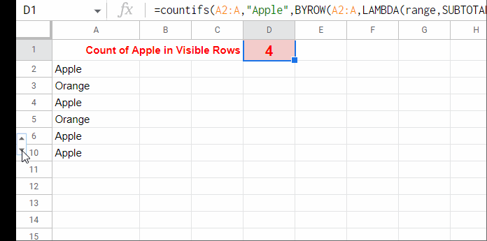
To utilize the BYROW function in Google Sheets to handle hidden rows, you can use the formula:

=BYROW(A2:A, LAMBDA(range, SUBTOTAL(103, range)))

(replace A2:A with any non-blank column reference within your range)

If you apply the above BYROW formula in cell E2, the formula will return 1 in all non-blank rows and 0 in blank rows.

Even if you hide any row through grouping, filtering, or manual hiding, the value returned by the above formula in the corresponding cell, though invisible, will be 0.

Therefore, I have employed the above BYROW formula within COUNTIFS in cell D1 to handle hidden rows as follows:

=COUNTIFS(A2:A, "Apple", BYROW(A2:A, LAMBDA(range, SUBTOTAL(103, range))), ">0")

To exclude all hidden rows (hidden through filtering, grouping, or manual hiding), use function number 103 within SUBTOTAL. If you want to only exclude rows hidden through filtering, replace 103 with 3.

Alternatively, you can use 9 or 109, but with numeric columns. Function numbers 103 and 3 work regardless of the column type.

Resources

Want to learn lambda helper functions other than the BYROW function in Google Sheets? Here you go!

1. How to Use the BYCOL Function in Google Sheets
2. How to Use the SCAN Function in Google Sheets
3. How to Use the REDUCE Function in Google Sheets
4. How to Use the MAP Function in Google Sheets
5. How to Use the MAKEARRAY Function in Google Sheets