


Let’s write a formula called ‘format rule’ to use in Conditional Formatting to highlight incorrect dependent text strings in Google Sheets.
To explain the topic, I am considering a table that contains a list of a few countries and their capital.
There are two columns, which are Country and Capital, as below.
| Country | Capital |
| Afghanistan | Kabul |
| Albania | Tirana |
| Algeria | Algiers |
| Andorra | Andorra la Vella |
| Angola | Luanda |
| Argentina | Buenos Aires |
| Armenia | Yerevan |
| Australia | Canberra |
| Austria | Vienna |
| Azerbaijan | Baku |
As per this two-column list, column B values are the dependents of column A values.
For example, “Canberra” is the dependent of “Australia”.
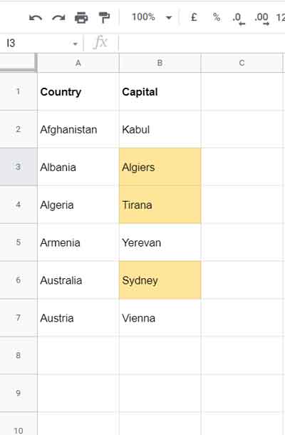
In another two-column list, if someone enters “Sydney” against “Australia”, I want to highlight “Sydney” as it’s the wrong dependent.
I have meant to convey this with the topic highlight incorrect dependent text in Google Sheets.
You can use the above example in your real life by replacing the table country and city with relevant values.
My formula will help you identify misaligned text strings by highlighting them.
Format Rules to Highlight Incorrect Dependent Text in Google Sheets
As per my test, we can use VLOOKUP or MATCH for writing the conditional format rule.
To highlight incorrect dependent text strings, first, create a table as above that contains proper alignment.
I have kept my above table in Sheet2!A1:B11.
I want to highlight the incorrect dependents in column B in Sheet1 in the same file.
Two Format Rules – Vlookup and Match
Let’s write the formulas from scratch.
Format Rule # 1 (Vlookup)
Since we are dealing with conditional formatting, we need to write the formula for the cell range A2:B2 in Sheet1. Based on the “Apply to range” A2:B1000, the same will apply to all the 1000 rows.
First, search the value A2&B2 (Sheet1) in the range Sheet2:A2:A11&Sheet2!B2:B11. The following Vlookup will do that part.
=ArrayFormula(vlookup(A2&B2,Sheet2!A2:A11&Sheet2!B2:B11,1,0))The ArrayFormula use is necessary as we are combining two arrays in Sheet2 using an ampersand.
At present, the conditional formatting in Google Sheets won’t support cross reference as above. We should use INDIRECT as below.
=ArrayFormula(vlookup(A2&B2,indirect("Sheet2!A2:A11")&indirect("Sheet2!B2:B11"),1,0))In any blank cell in Sheet1, this formula will return #N/A if there is no match, else the combined value.
To highlight incorrect dependent text, we require the #N/A values.
Using the IFNA function, we can convert #N/A values to TRUE (a Boolean value equal to # 1). It’s as follows.
=ifna(ArrayFormula(vlookup(A2&B2,indirect("Sheet2!A2:A11")&indirect("Sheet2!B2:B11"),1,0)),TRUE)It is not enough for highlighting!
Because we want to use the format rule in an entire column range in Sheet1, not only in B2.
There may be blank rows in B2:B in Sheet1, for which also the VLOOKUP will return #N/A error values.
To overcome that issue, we can use the AND operator as below.
=and(len(B2),ifna(ArrayFormula(vlookup(A2&B2,indirect("Sheet2!A2:A11")&indirect("Sheet2!B2:B11"),1,0)),TRUE)=TRUE)We can use the above format rule to highlight incorrect dependent text in Google Sheets.
Here is one more formula for educational purposes.
Format Rule # 2 (Match)
Like format rule # 1, we can also write another rule using MATCH to highlight misaligned text strings in Google Sheets.
Here, I am giving you the formula straight away.
=AND(LEN(B2),ifna(ArrayFormula(match(A2&B2,indirect("Sheet2!$A$2:$A$11")&indirect("Sheet2!$B$2:$B$11"),0)),TRUE)=TRUE)Here the formula works similar to Vlookup. Let’s see how?
The below formula part would also return #N/A for the mismatch. Instead of the combined value, this formula would return the relative position number for the match.
=ArrayFormula(match(A2&B2,indirect("Sheet2!$A$2:$A$11")&indirect("Sheet2!$B$2:$B$11"),0))The rest of the parts are similar to Vlookup. I mean, use IFNA to convert #N/A to TRUE and use the AND to skip blank cells.
We have two format rules now. I am using the first rule, and let’s see how it highlights incorrect dependent text string.
How Do I Implement the Format Rule?
Please follow the below steps.
1. Copy the format rule # 1.
2. In Sheet1, select B2:B1000 or the number of rows that you want in the range B2:B.
3. Click Format > Conditional formatting.
4. On the format editor (Conditional format rules panel), please check the “Apply to range” field. It will be B2:B1000 or the selected range. If not, correct it.
5. Under Format rules, pick “Custom formula is” and paste the copied formula in the blank field.
6. Select the color to highlight (light yellow as per my example) and click “Done”.
This way, we can highlight incorrect dependent text strings in Google Sheets.
That’s all!
Thanks for the stay. Enjoy!