Using the GETPIVOTDATA function we can get a single value from any row or column from a Pivot Table in Google Sheets.

At present, it’s the one and the only function in Sheets to get a single value from a Pivot Table.

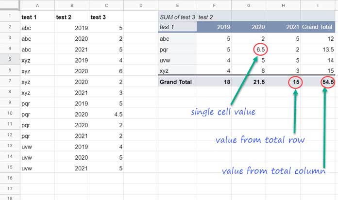
Assume you have a Pivot Table in the range E1:I7. You may not use =G4 to get the value from cell G4. It may land you in problems.

It will, of course, return the value from the cell in question. But most probably, any update in the PT (Pivot Table) source will affect the result.

Using GETPIVOTDATA, we can specify relationships between data points in Sheets. So we will always get the correct value irrespective of any update in the source.

You may know how to get a single value from the total row or column of a Pivot Table.

What about a single cell not in the total row?

This post has answers to all of these.

Before further proceeding, please note one thing.

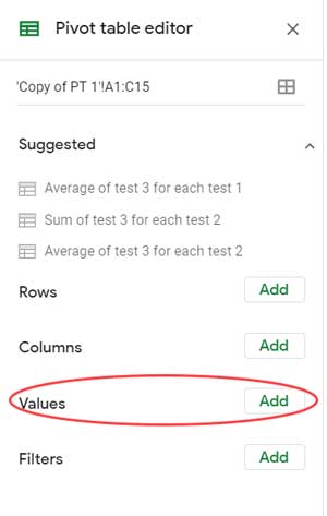
From my understanding, to use the GETPIVOTDATA function in Google Sheets, your PT has the “Values” field in use.

Some people use PT to just filter source data. In such a case, if you try to use the said function, you may see the error #REF!.

Field combination not found in pivot table for function GETPIVOTDATA

If your purpose is filtering a range, then use FILTER, QUERY, or the SLICER.

Getting Single Value from a Pivot Table in Google Sheets

You won’t be using the same type of PT that I am using. So to make you understand, I am going to give examples of two different PTs.

Please see image # 1 above. I have data in columns A, B, and C. Using that data, I have created a Pivot Table and that also you can see on the same image in the range E1:I7.

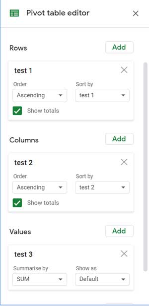
Here are the settings in use for the same.

Value Name

Now, most importantly, to get a single value from the above Pivot Table in Google Sheets, make sure that it has the “Values” field in use. My above PT satisfies this condition.

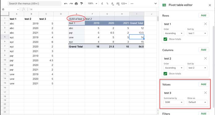
The field used in “Values” is “test 3”, and the function in use is SUM. Please see image # 3 above. So, in the PT report, you will see the “Value Name” field as SUM of test 3″.

If you could understand this, using the GETPIVOTDATA will become child’s play. The reason for this is, the Value_Name is the first and most important argument in the above function.

Syntax: GETPIVOTDATA(value_name, any_pivot_table_cell, [original_column, …], [pivot_item, …])

Four Formula Examples to Learn to Get a Single Value from a Pivot Table in Google Sheets

I’ve already explained all the necessary points that you should know before going to the formulas.

Formula 1

Assume I want to get the value in cell G4 from the above Pivot Table report.

How to get it using the GETPIVOTDATA function?

Here is that formula.

=GETPIVOTDATA("Sum of test 3",E1,"test 2",2020,"test 1","pqr")

This formula will return the required cell value from the PT report. How?

value_name: “Sum of test 3”.

– I have already explained this parameter.

any_pivot_table_cell: E1.

– The PT range is E1:I7. So used E1, you can use any cell from this range

original_column: “test 2”.

– You can see three columns in the pivot table report, i.e., 2019, 2020, 2021. They are not columns but “pivot_items”. The column is “test 2”.

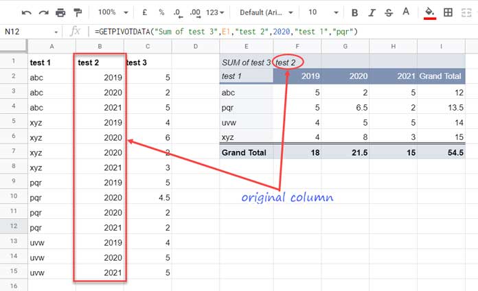
pivot_item: 2020.

We want to get a single value from the Pivot Table in cell G4. It is under the column “test 2” and below the “pivot_item” 2020.

Additional Arguments (original_column_2 and pivot_item_2):

original_colum_2: “test 1”, pivot_item_2: “pqr”.

The value to extract (in G4) is against the item “pqr” (in E4) which is under the original column “test 1”.

Now we can play around with this formula to get value from any cell in the Pivot Table in Google Sheets.

Formulas 2 to 4

Formula # 2:

GETPIVOTDATA formula to get the value 13.5 (in I4) under the “Grand Total” column against “pqr”:

=GETPIVOTDATA("Sum of test 3",E1,"test 1","pqr")

value_name: “Sum of test 3”.

any_pivot_table_cell: E1.

original_column: “test 1”.

pivot_item: “pqr”.

Formula # 3:

GETPIVOTDATA formula to get the value 21.5 in cell G7 in the “Grand Total” row:

=GETPIVOTDATA("Sum of test 3",E1,"test 2",2020)

Formula # 4:

GETPIVOTDATA formula to get the Grand Total value 54.5 in cell I7.

=GETPIVOTDATA("Sum of test 3",E1)

Conclusion

At the beginning of this tutorial, I have promised to give formulas based on two pivot tables. Above I have already elaborated one.

I am attaching a sample sheet herewith. In that sheet, in the tab “PT 1”, you can see all the above examples.

There is one more sheet tab named “PT 2”.

Please refer to that tab to get more formulas.

Sample_Sheet_19321

I hope you could understand how to get a single value from a Pivot Table in Google Sheets.

That’s all.

Thanks for the stay. Enjoy!

Related:

• Extract Total and Grand Total Rows From a Pivot Table in Google Sheets.