To find the closest match in an array of numeric values in Google Sheets, we can use the Filter, Min, and Abs functions combo.
There is one more popular method among Excel users, which works in Google Sheets too.
In that method, we replace Filter with Index-Match. It has one issue, though!
What’s that?
If there are two closest matches, one higher value and one lower value, the formula will only return the lower value.
But the Filter, Min, and Abs combo can return both values. I’ll elaborate the same under the example below.
Formulas to Find Closest Match in Google Sheets
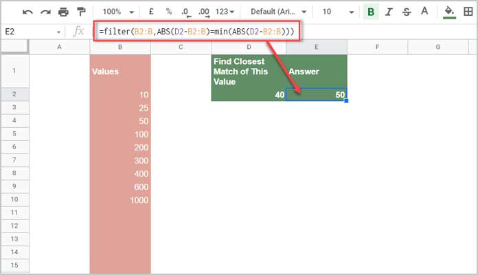
Sample Data: B1:B (where B1 contains column name)
Value to Evaluate in Sample Data: D2
Formula to Find Closest Match:
Insert either of the below formulas in cell E2.

Formula # 1 (Filter [Google Sheets] Approach):
=filter(B2:B,ABS(D2-B2:B)=min(ABS(D2-B2:B)))Formula # 2 (Index-Match [Excel] Approach):
=index(B2:B10,match(min(ABS(D2-B2:B10)),ABS(D2-B2:B10),0))Using the above formulas, we can find the closest match of the value in cell D2 in the array B2:B.
Change the value in D2 to 500 and find the closest value using both the formulas.
The first formula will return two values. They are 400 and 600.
The second one will return only one value, i.e., 400.
Formula Explanations
Formula 1 – Filter Approach
It’s essentially a FILTER formula.
Syntax: FILTER(range, condition1, [condition2, …])
In this, we know the range to Filter is B2:B. What about argument condition1?
It’s ABS(D2-B2:B)=min(ABS(D2-B2:B))
We can split this condition1 into two parts.
Part_1: ABS(D2-B2:B)
Part_2: min(ABS(D2-B2:B)) or we can say min(part_1).
What do the part_1 and part_2 formulas return then?
We can test them in a Sheet (using ArrayFormula with them is a must outside Filter).
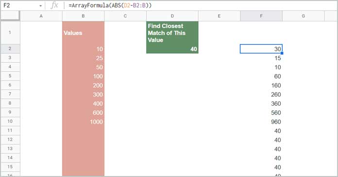
Part_1 Test in Cell F2:
=ArrayFormula(ABS(D2-B2:B))
The part_1 returns the difference of numbers in B2:B from D2, i.e., D2-B2:B.
Note:- I have used ABS, i.e., ABS(D2-B2:B), to return the absolute numbers (numbers without -ve sign).
By wrapping the above formula with MIN, we can get the min value difference, i.e., part_2.
That is the key to finding the closest match in Google Sheets.
Part_2 Test in Cell G2:
=ArrayFormula(MIN(ABS(D2-B2:B)))Output: 10
It’s the third number in cell range F2:F (part_1).
If we filter B2:B (range) using the condition F2:F=G2 (part_1=part_2), we will get 50.
This way, we can find the closest match in Google Sheets.
Formula 2 – Index-Match Approach
If you could understand how to use the Filter, Min, and Abs combo to find the closest match in Google Sheets, the Index-Match way of doing the same is simple to learn.
Here also we will use the above part_1 and part_2 for explanation purposes.
In this approach, I have used the MATCH function to find the (relative) position of part_2 output in part_1 output.
Then using INDEX, I have managed to offset that many rows in B2:B to get the closest match.
Finding the Closest Match in Google Sheets and Its Real-Life Use
For example, you are one of the suppliers of landscaping materials, and you have a stock of 20-40 mm white pebbles.
Assume, the unit price of this item varies based on the order quantity.
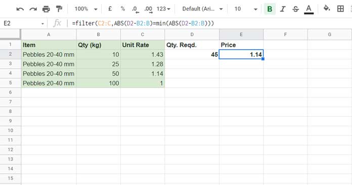
I mean, for the order quantity of 10 kg, you sell the item at 1.43 per kg.
If the order quantity is 25 kg, then you sell the same item at 1.28 per kg.
The unit rate is 1.14 for 50 kg and 1 for 100 kg.
You want to find the closest unit price when someone orders 45 kg.
In this case, you can use one of my above formulas, which finds the closest match in Google Sheets. Here is how.
=filter(C2:C,ABS(D2-B2:B)=min(ABS(D2-B2:B)))
The formula finds the closest match of quantity and returns its unit price.
Resources
- Find the Past or Future Closest Date to Today in Google Sheets.
- Query to Filter Closest Higher Date to Today in Google Sheets.
- Nearest Match Greater Than or Equal to Search Key in Vlookup in Google Sheets.
- Alternatives to the XMATCH Function in Google Sheets.
- XLOOKUP Alternatives in Google Sheets – Search and Match Modes.
- How to Lookup Latest Dates in Google Sheets [Array Formula].
- Extract the Earliest or Latest Record in Each Category Based on Timestamp.
- Lookup Latest Value – How It Differs in Excel and Google Sheets.
- Formula to Combine Rows and Get Latest Values in Google Sheets.


