As you may know, filtering rows with merged cells in columns in Google Sheets often doesn’t yield the desired results. What’s the solution?

There are two main options for filtering a table or data set: using built-in tools or native Google Sheets functions.

When using functions, you will only get the first row of the merged cells.

However, when using built-in tools like Slicer or Create a filter in the Data menu, the issue used to be that it would return the error “You can’t create a filter over a range containing vertical merges.” This seems to have been resolved.

The functions with advanced filtering capabilities are FILTER and QUERY. Let’s look at an example using these functions to understand the issue.

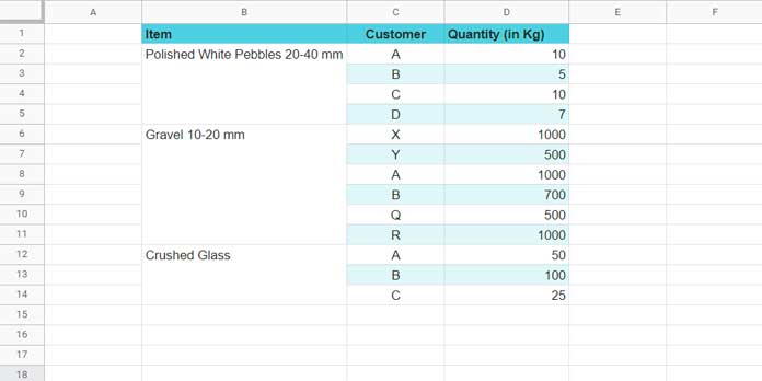
I have a three-column data set containing Item, Customer, and Quantity (in Kg) in columns B, C, and D, respectively.

I want to filter all customers who require Polished White Pebbles 20-40 mm. You can try the following FILTER or QUERY formulas:

Filter:

=FILTER(
   B2:D, 
   B2:B = "Polished White Pebbles 20-40 mm"
)

Query:

=QUERY(
   {B2:D}, 
   "SELECT * WHERE Col1 = 'Polished White Pebbles 20-40 mm'"
)

These formulas will return only the first row in the range, i.e., data in B2:D2, when we expect B2:D5. This is because B2:B5 is merged and B2 contains the required item, leaving B3:B5 empty.

So, what is the solution to properly filter data when the criteria column contains vertically merged cells using these functions in Google Sheets?

Filter Rows with Merged Cells in a Column in Google Sheets

The first step is to create a helper column containing an array formula that fills the merged cells with the values from the cell above.

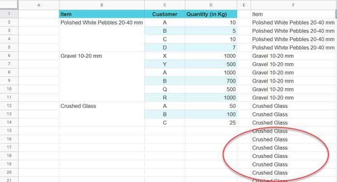
In our sample data, the merged range is B2:B, and the data range is B2:D. So, you should apply the formula, preferably in cell F2, after clearing the contents of F2:F.

You can then use that helper column directly with the FILTER or QUERY functions. If you prefer not to use a helper column, you can incorporate the formula within these functions directly. I’ll cover that later on.

Preparing the Helper Column

In cell F2, insert the following LOOKUP formula to fill merged cells down the column:

=ArrayFormula(LET(range, B2:B, LOOKUP(ROW(range), ROW(range)/(range<>""), range)))

Before filtering data based on a condition in column B, which contains merged cells, we need to address one issue.

The data in the table ends at row 14, as you can see by looking at columns C or D. However, the formula fills the last value in column B all the way down. We need to restrict this.

There are three options to remove these unwanted values.

Options to Remove Unwanted Strings:

1. Use the closed range B2:B14 instead of B2:B in the F2 formula.
2. Go to cell B15 and tap the spacebar. This way, you won’t need to make any changes to the above LOOKUP formula in cell F2.
3. Replace the range B2:B with INDIRECT("B2:B"&XMATCH(TRUE, C2:C<>"", 0, -1)).

Note: The XMATCH part of the formula in option 3 returns the row number of the last non-empty cell in column C.

If you follow the third option, the F2 formula will become:

=ArrayFormula(LET(range, INDIRECT("B2:B"&XMATCH(TRUE, C:C<>"", 0, -1)), LOOKUP(ROW(range), ROW(range)/(range<>""), range)))

Filtering Data with Criteria from Vertically Merged Cells in a Column

It’s formula time.

The following FILTER formula will filter the range B2:D where F2:F is equal to “Polished White Pebbles 20-40 mm”:

=FILTER(
   B2:D, 
   F2:F = "Polished White Pebbles 20-40 mm"
)

Here’s the equivalent QUERY formula:

=QUERY(
   {B2:D, F2:F}, 
   "SELECT Col1, Col2, Col3 WHERE Col4 = 'Polished White Pebbles 20-40 mm'"
)

This method allows you to filter data when the criteria column contains merged cells.

If you prefer not to use a helper column, you can incorporate the formula from F2 directly within the functions.

In both the FILTER and QUERY formulas, replace F2:F with the formula from the “Preparing the Helper Column” section that does not include the XMATCH function.

Resources

• Copy-Paste Merged Cells Without Blank Rows/Spaces in Google Sheets
• Uncover Merged Cell Addresses in Google Sheets
• How to Merge Two Columns Into One Column in Google Sheets
• How to Use SUMIF in Merged Cells in Google Sheets
• Sort Vertically Merged Cells in Google Sheets (Workaround)
• Sequence Numbering in Merged Cells In Google Sheets
• How to Use SUMPRODUCT with Merged Cells In Google Sheets
• How To Use COUNTIF or COUNTIFS In Merged Cells In Google Sheets
• How to Use VLOOKUP in Merged Cells in Google Sheets
• XLOOKUP in Merged Cells in Google Sheets
• Creating Sequential Dates in Equally Merged Cells in Google Sheets