To calculate the cumulative interest payment for an investment in Google Sheets, you can utilize the CUMIPMT function.
This function shares similarities with another financial function in Google Sheets, namely IPMT (interest payment). I’ll elucidate the distinctions between CUMIPMT and IPMT.
Like IPMT, the CUMIPMT function is applicable only if your investment adheres to the following conditions:
- Constant-amount periodic payments.
- Constant interest rate.
Syntax:
CUMIPMT(rate, number_of_periods, present_value, first_period, last_period, end_or_beginning)Arguments:
Please note that there are no optional arguments in the Google Sheets CUMIPMT function, so you must include all the following arguments in the formula:
rate: The interest rate.number_of_periods(Nper): The total number of payment periods.present_value(Pv): The present value of the investment/annuity.first_period: The starting period (cumulative range starting) in the calculation. It must be greater than or equal to 1 and less than or equal tolast_period.last_period: The end period in the calculation. It must be greater than or equal tofirst_periodand less than or equal to Nper.end_or_beginning: The timing, i.e., whether the payments are due at the end (represented by the number 0) or beginning (represented by the number 1) of each period, of the payment.
Note:
If the first period and the last period in the CUMIPMT function in Google Sheets are the same, it will return the IPMT of that period. I will explain after presenting the CUMIPMT formula example below.
Formula Example of the CUMIPMT Financial Function in Google Sheets
In the example below, I have calculated the cumulative interest payment of a loan from the first period to the last period.
Data in A1:B6, where A1:A6 contains descriptions and B1:B6 contains the values to use in the formula.
| Loan Amount (Pv) | 25000 |
| Interest Rate (Annual) | 4.5% |
| Loan Period (Nper) | 2 |
| First Period | 1 |
| Last Period | 24 |
| End or Beginning | 0 |
This loan is for 2 years and is paid monthly, resulting in 24 periodic payments.
CUMIPMT Formula:
=CUMIPMT(B2/12, B3*12, B1, B4, B5, B6) // returns -1188.69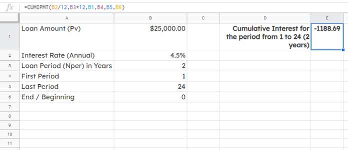
To obtain the cumulative interest payment for a different period range, such as period 13 to 24, change B4 to 13 and B5 to 24. No changes are needed in the formula since we use cell references.
The cumulative interest payment for the second year (period 13 to 24) will be -313.67, as per the above example.
As observed above, the CUMIPMT formula output in Google Sheets is a negative number due to cash outflow. If you want to change the sign, wrap the CUMIPMT formula with UMINUS, as shown below:
=UMINUS(CUMIPMT(B2/12, B3*12, B1, B4, B5, B6)) // returns 1188.69Important Note:
In the formula, it is crucial to use consistent units in two arguments, specifically the interest rate and number of periods (Nper).
For instance, if the loan amount is for 2 years with monthly payments, divide the interest rate by 12 to obtain the monthly interest rate and multiply Nper by 12.
If the provided interest rate in cell A2 is already a monthly interest rate, then there is no need to divide it by 12.
Similarly, if the number_of_periods (Nper) is provided in the number of months instead of the number of years, there is no need to multiply the value in cell B3 by 12.
Related Reading: How to Use the NPER Function in Google Sheets
CUMIPMT vs IPMT in Google Sheets
I have already provided a detailed explanation of the IPMT function in a separate tutorial. However, for comparison, here is an example of an IPMT formula based on the previously mentioned sample data.
Syntax (IPMT):
IPMT(rate, period, number_of_periods, present_value, [future_value], [end_or_beginning])Formula to find the interest payment for period 1:
=UMINUS(IPMT(B2/12, 1, B3*12, B1, 0, 0)) // returns 93.75The interest payment for the last period (24) will be calculated as follows:
=UMINUS(IPMT(B2/12, 24, B3*12, B1, 0, 0)) // returns 4.08Similarly, using the IPMT function, you can calculate the interest payment for any period. The interesting fact is that you can even use CUMIPMT to calculate the interest payment for any single period! For that, use the same number in both the first period and the last period.
For instance, to calculate the interest for the final period (24), enter 24 in both cells B4 and B5. Without a doubt, the output will be $4.08, consistent with the IPMT result mentioned earlier.
Creating Cumulative Interest Payment Schedule in Google Sheets
To generate an array result or, in other words, a cumulative interest payment schedule, input the numbers 1 to 24 (representing 24 periods, as per the sample data above) in the last period. How?
Simply replace the last period (B5) in the CUMIPMT formula with ROW(A1:A24). The ROW formula returns sequential numbers from 1 to 24.
Note: In all the formulas below, you can replace ROW(A1:A24) with SEQUENCE(24). SEQUENCE was not available when I first coded these formulas.
Set the B4 value (first period) to 1. Additionally, enclose the entire formula with ArrayFormula.
=ArrayFormula(UMINUS(CUMIPMT(B2/12, B3*12, B1, 1, ROW(A1:A24), B6)))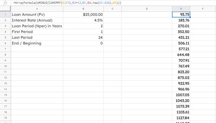
The above formula represents a cumulative interest payment schedule. To obtain the amount for each period separately, use this array formula in cell D1.
=ArrayFormula(UMINUS(IPMT(B2/12, ROW(A1:A24), 24, B1, 0, 0)))Conclusion
In this tutorial, we explained how to use the CUMIPMT function to calculate the cumulative interest payment for an investment in Google Sheets. Additionally, we demonstrated its use with array formulas and ROW/SEQUENCE to create a cumulative interest payment schedule. Before concluding, here’s one more tip:
Wrap the aforementioned IPMT array formula with the SUM function as shown below.
=SUM(ArrayFormula(UMINUS(IPMT(B2/12, ROW(A1:A24), 24, B1, 0, 0))))This IPMT formula is equivalent to the following CUMIPMT formula and is useful for overcoming the current limitation of a maximum of 999 periods in CUMPIMPT.
=UMINUS(CUMIPMT(B2/12, B3*12, B1, 1, 24, B6))That’s all. Enjoy!


