The IPMT function in Google Sheets helps calculate the interest portion of a payment for an investment or loan during a specific period. The ‘I’ in IPMT stands for interest.
You should use the IPMT function to calculate the interest payment only if the loan or investment is based on constant, periodic payments and a fixed interest rate. This condition is essential.
To calculate the total payment (including both principal and interest) for an investment or loan, you can use the PMT function, which I’ve previously covered in this blog.
Once you have the total payment (PMT), you can separate the interest portion using the IPMT function for any period within the duration of the loan.
What about the principal portion?
For the principal payment portion, there’s another function that I will explain in a future tutorial.
Syntax of the IPMT Function in Google Sheets
Syntax:
IPMT(rate, period, number_of_periods, present_value, [future_value], [end_or_beginning])- rate: The annual interest rate.
- period: The specific period for which you want to calculate the interest.
- number_of_periods (Nper): The total number of payments to be made.
- present_value (Pv): The current value of the loan or investment.
- future_value (Fv): Optional, default is 0. It represents the balance remaining after the last payment.
- end_or_beginning: Optional, default is 0. It determines whether payments are due at each period’s end (0) or the beginning (1).
Calculating the Interest Portion of a Loan Payment in Google Sheets
Let’s go through an example of how to use the IPMT function. First, we’ll calculate a home loan’s monthly payment (EMI) using the PMT function.
Sample Data in Cells A1:B3:
- Interest rate (annual mortgage rate): 4%
- Number of periods (loan term in years): 30
- Loan amount: $100,000
Formula to calculate EMI:
=PMT(B1/12, B2*12, B3)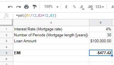
The monthly EMI for this loan is -$477.42. This payment includes both the principal and interest.
Now, using the IPMT function, we can isolate the interest portion from this payment. Here’s how to calculate the interest for the first payment (the first month’s installment):
Monthly Interest Using the IPMT Function
The IPMT formula is similar to the PMT formula, with one key difference: you need to specify the period for which you want to calculate the interest.
Sample Data in Cells A1:B4:
- Interest rate (annual mortgage rate): 4%
- Period: 1
- Number of periods (loan term in years): 30
- Loan amount: $100,000
Formula:
=IPMT(B1/12, B2, B3*12, B4)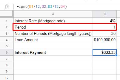
This formula returns -$333.33, meaning that out of the total payment of -$477.42, $333.33 is the interest for the first month.
As you may notice, the interest amount is higher at the beginning of the loan and gradually decreases over time.
Curious about the interest on the final payment?
Simply change the value in cell B2 from 1 to 360. This is because the loan term is 30 years, and since payments are monthly, there are 360 total payments (30 years × 12 months).
For the 360th payment, the interest portion is a mere $1.59!
Quarterly Interest Calculation Using the IPMT Function
If your loan has quarterly payments instead of monthly payments, you can adjust the formula accordingly. In this case, divide the annual interest rate by 4 (for quarterly periods) and multiply the number of periods by 4.
Formula:
=IPMT(B1/4, B2, B3*4, B4)In this example, the interest portion of the first quarterly loan repayment is $1,000.
Yearly Interest Calculation Using the IPMT Function
For yearly payments, you don’t need to divide or multiply the interest rate and periods. You can use the formula as-is:
=IPMT(B1, B2, B3, B4)This method allows you to calculate the interest portion of yearly payments directly.
Conclusion
The IPMT function in Google Sheets is a powerful tool for breaking down the interest portion of your loan or investment payments. By adjusting the formula based on your payment frequency (monthly, quarterly, or yearly), you can easily calculate interest for any period. Thanks for reading, and happy calculating!


