Using Filter and Textjoin, we can easily concatenate header names with the values of the cells below them in Google Sheets. But it would be a non-array (drag-drop) formula.
Using a Query and IF (the two key functions in the formula) based array formula, we can achieve the same type of concatenating array result in Google Sheets.
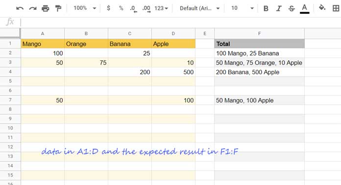
Let me start by explaining the problem in detail. For that, we can depend on the below table range A1:D.

My data table is in the range A1:D and in that some of the cells have values and some of them don’t have.
I just want to get the result as per the data in F1:F.
That means I want to get the header names concatenated with the non-blank cells below them.
If any cell is blank, I don’t want the corresponding header name in the output.
I can further clarify it.
For explanation purposes, we can consider the header names in A1:D1 and the values in A2:D2. Let’s forget about other rows (A3:D) for the time being.
If we concatenate the header names with the values of the cells below them in A2:D2, I want to get “100 Mango, 25 Banana” instead of “100 Mango, Orange, 25 Banana, Apple”.
I hope, you could understand the difference.
Formulas to Concatenate Header Names with the Values of the Cells Below Them
How to concatenate header names with the values of the cells below them in Google Sheets?
Let me explain.
As I have mentioned, I have an array formula and a non-array formula. You can choose either of the ones depending on the volume of your data.
Since it’s simple to explain the non-array version, I’ll start with that.
If you already know how to use a non-array formula to combine header names with the non-blank cells below them, then you can skip the following non-array formula part.
Non-Array Formula Using Filter and Textjoin
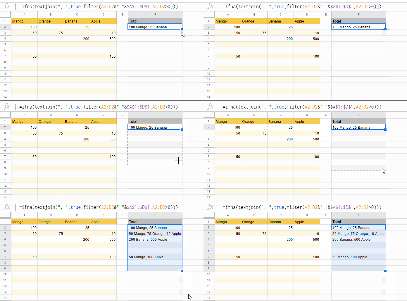
In F2, key in the following non-array formula.
=ifna(
     textjoin(
        ", ",
        true,
        filter(A2:D2&" "&$A$1:$D$1,A2:D2>0)
     )
)
Then copy and paste down (drag the fill handle [blue square at the edge] down as shown below).

In this formula, you should understand the Filter first.
The first part of the Filter formula (filter range) is A2:D2&" "&$A$1:$D$1.
It will return the below result.
| 100 Mango | Orange | 25 Banana |
The above is the ‘range’ in Filter.
Note: If you attempt the above formula in any cell, like =A2:D2&" "&$A$1:$D$1, it would return #VALUE! error. Because in standalone use (outside Filter use), the ampersand sign with ranges/arrays require the ArrayFormula like =ArrayFormula(A2:D2&" "&$A$1:$D$1).
Syntax of the Filter for your Quick Reference:
FILTER(range, condition1, [condition2, …])The Filter filters the ‘range’ if the values in A2:D2 is greater than 0. So the result would be the first and the last item from the ‘range’.
The Textjoin joins these two values and places a comma delimiter in between.
The IFNA in the formula is to return blank (while dragging-down) if any row is totally blank.
That’s all about the non-array formula to concatenate header names with the non-blank cell values below them in Google Sheets.
Array Formula Using IF and Query as the Key Functions
Formula:
=ArrayFormula(
     {"Total";
        REGEXREPLACE(
           trim(
              transpose(
                 query(
                    transpose(if(A2:D<>"",A2:D&" "&A1:D1&",",)),,
                    9^9
                 )
              )
           ),
           "(.)\z",""
        )
     }
)
Simply insert this formula in cell F1 (if F2:F is blank, else empty F2:F first) to cover the range A1:D. So we can call it an array formula. No hassle of drag-drop the fill handle.
How this array formula concatenate headers with the values of the cells (range) below them in Google Sheets?
Please Go through the formula explanation below.
Part_1_Formula
There are two main parts to the formula. Here I am starting with the IF formula part.
Please note that unlike in the master formula, you may see the ArrayFormula function use here. It’s mandatory in a standalone use.
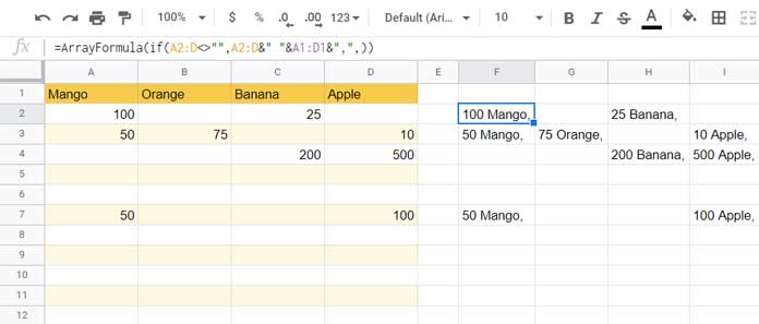
=ArrayFormula(if(A2:D<>"",A2:D&" "&A1:D1&",",))
The IF formula combines the headers with the values below them. But the values are placed in multiple columns, not in a single column as per our requirement.
We want the combined values corresponding to A2:D2 in F2, A3:D3 in F3, and so on. The formula part two takes care of that.
Part_2_Formula
We can use Query to join columns in Google Sheets.
For that, just Transpose the above IF result, and Query it and again Transpose it.
Here is the Generic Formula.
Generic Formula:
=transpose(query(transpose(Part_1_Formula),,9^9))Here is the Part_2_Formula as per the above generic formula and its result.
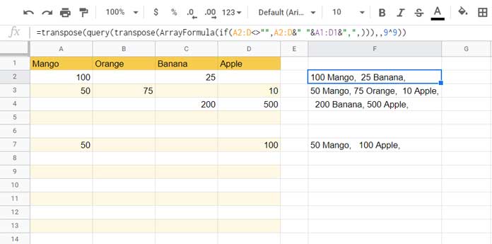
=transpose(query(transpose(ArrayFormula(if(A2:D<>"",A2:D&" "&A1:D1&",",))),,9^9))
The above formula itself is enough to concatenate header names with the values of the cells below them.
But the result is not perfect as it contains extra white spaces and additional delimiters at the end.
In the final formula, the TRIM removes the extra white spaces, whereas the Regex removes the additional delimiter from the end.
Further, the ArrayFormula inside moved to the outer part.
That’s all. Enjoy!


Does this formula work in Excel for Windows? If so, how do I use it in the way “Mango:100, Orange:25, and so on…
Thanks!
Hi, Goulart,
The filter formula will work in Excel for Microsoft 365 after making a few changes.
Try this.
=IFERROR(TEXTJOIN( ", ", TRUE,FILTER(A2:D2&": "&$A$1:$D$1,A2:D2>0)),"")Hi, this is exactly what I was looking for, but there is one issue that I am experiencing. It is dropping the last character of the last entry.
LOL, the issue with the output is that after the first header, all following headers have a space inserted in front of them, making the output offset.
Hey, Tommy!
Did you find a way to fix the issue of the last character being trimmed??
Hi, Judd,
I couldn’t replicate the issue! So, can you please consider sharing the URL of a mockup sheet in your reply below?