


In my sum by month tutorial, one of my readers asked me about the formula for average by month in Google Sheets.
Since I have an array and multiple non-array formulas, I am writing the answer to him as a new tutorial. This post is the answer.
I hope this will help other readers also who like to learn new things in Google Sheets.
To calculate the average by month in Google Sheets, we can use AVERAGEIF, FILTER + AVERAGE, and QUERY.
There may be other solutions too. But I am limiting to these three types of formulas.
Among the formulas, the first two are non-array formulas, and the last one is an array formula.
Let’s start with the non-array formulas.
Average by Month in Google Sheets (Non-Array Formulas)
As I have mentioned above, there are two types of non-array formulas that you will get below. Both formulas are for different purposes.
You can find more details about the formula results below.
Averageif Formula
In cell range B2:B7, enter the dates 25/11/2020, 26/11/2020, 1/12/2020, 6/12/2020, and 21/12/2020.
In the next column in the corresponding cells, i.e., in the cell range C2:C7, enter the numbers 5, 4, 5, 6, 5, and 11.
We can use the AVERAGEIF function as below to return the average by month in Google Sheets.
To get the average for November month, we can use the below formula.
=ArrayFormula(IFERROR(averageif(month($B$2:$B),11,$C$2:$C)))Even though it’s not an array formula, we have used the ArrayFormula function since we have used the MONTH function in a range in the formula.
For December month’s average, replace criterion 11 in the formula with 12.
=ArrayFormula(IFERROR(averageif(month($B$2:$B),12,$C$2:$C)))In real-life use, you can specify the criteria in the range E2:E13 as below and then use the below formula in cell F2, then drag it down.
=ArrayFormula(IFERROR(averageif(month($B$2:$B),E2,$C$2:$C)))
Though the above formula is easy to read even by a beginner, it has one drawback!
What’s that?
In the above AVERAGEIF based formula, we can’t include the year part.
I mean, if your data has values in January 2020 and January 2021, the above formula would only consider the month part.
The reason, the AVERAGEIF formula only supports one criterion. So we can’t include the year part in the formula.
Then can we use the AVERAGEIFS?
Nope! Because the criteria month and year are in the same date column. As far as I know, the AVERAGEIFS won’t support it.
If you want to include month and year in the month-wise average calculation in Google Sheets, then use the Filter + Average combo as below.
Average by Month and Year Using Filter and Average
I am modifying the data to accommodate values in multiple years.
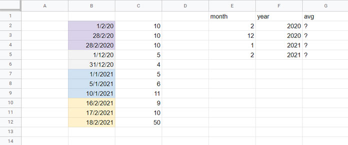
Earlier, the data was in B2:C6. The new data range is B2:C12.
Here are the steps to write the formula that returns average by month and year in Google Sheets.
Let’s first consider the month number 2 (February) in cell E2 and the year 2020 in cell F2.
Using Filter, we should first filter the range C2:C that falls in the month range of February 2020 in cell range B2:B.
=FILTER($C$2:$C,month($B$2:$B)=E2,year($B$2:$B)=F2)The above Filter formula filters the values as per the criteria given.
Enclose it within the AVERAGE function as below.
=average(filter($C$2:$C,month($B$2:$B)=E2,year($B$2:$B)=F2))We can use the above Filter + Average formula in cell G2 to return the average by month (February) and Year (2020) in cell G2.
Drag this formula down to G5, and voila!
Average by Month and Year Using Query in Google Sheets (Array Formula)
If you are searching for an array formula to average by month and year in Google Sheets, no doubt, the function Query has no replacement.
You May Like: How to Sum, Avg, Count, Max, and Min in Google Sheets Query.
But many Google Sheets users seem hesitant to use Query as they might think it’s somewhat complicated. On the contrary, from my own experience, Query is simple to use and read.
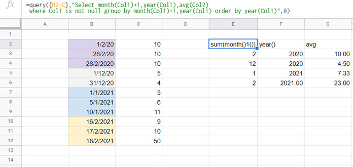
To average by month and year, we can use the below ‘unformatted’ Query formula.
=query({B2:C},"Select month(Col1)+1,year(Col1),avg(Col2) where Col1 is not null group by month(Col1)+1,year(Col1) order by year(Col1)",0)I have called it ‘unformatted’ as I haven’t customized the default labels returned by the Query in the first row of the result. Please see the below image (E2:G2).
Formula Explanation
Here let me explain the Query formula parts so that you can easily read them and use them.
SELECT Clause Part:-
Select month(Col1)+1,year(Col1),This Query formula part returns the values in the result columns E (months) and F (years).
Why I used month(Col1)+1 instead of using month(Col1) to return the month numbers?
It’s a natural question any reader may ask. The reason is the month numbers returned by Query are 0-11, not 1-12.
AVG Aggregation Part:-
avg(Col2)Needles to say, it is to perform the average aggregation in the second column in the range.
WHERE Clause Part:-
where Col1 is not nullWe have used the infinite range B2:C, not the finite range B2:C12, in our above average by month and year Query. So, there would be several blank rows.
The above clause excludes the blank rows in the range.
GROUP BY Clause Part:-
group by month(Col1)+1,year(Col1)We want to group by month and year.
ORDER BY Part:-
order by year(Col1)To sort by year.
If you want you can include LABEL CLAUSE to modify the labels in the result.
Example:
=query({B2:C},"Select month(Col1)+1,year(Col1),avg(Col2)
 where Col1 is not null group by month(Col1)+1,year(Col1) order by year(Col1) label month(Col1)+1'Month'",0)
You May Like: What is the Correct Clause Order in Google Sheets Query?
Average by Month Name in Google Sheets (Query)
In all the above examples, the formula returned month numbers, not month name text.
Many of you may wish to get the month names instead of the month numbers in the average by month and year formula results in Google Sheets.
We can do that using a simple Query trick. Here is the logic.
We will convert the dates to the end of the month dates. So, instead of grouping months, we can group the date column directly.
It avoids the use of the month function in Query.
See the below Query (just read until the next formula).
=Query({ArrayFormula(if(B2:B="",,eomonth(B2:B,0))),C2:C},"Select Col1,avg(Col2) where Col1 is not null group by Col1",0)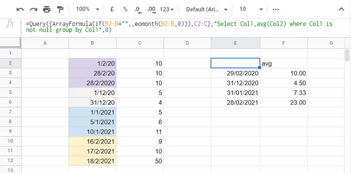
Note:- If you use the above formula, you would see date values in E3:E6, not the dates, as shown in the image. I have formatted the date-values to date from the menu Format > Number > Date. It is to make you understand the purpose of the end of the month conversion.
We can use the FORMAT clause in the above Query to format the column 1 (E3:E6) values to month and year as below.
=Query({ArrayFormula(if(B2:B="",,eomonth(B2:B,0))),C2:C},"Select Col1,avg(Col2) where Col1 is not null group by Col1 format Col1'mmmm-yyyy'",0)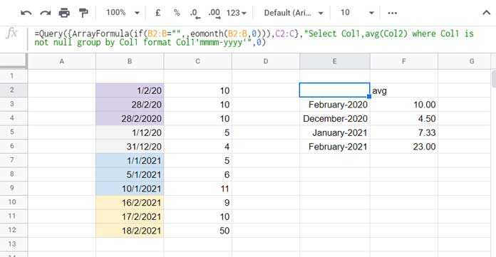
I hope you could understand how to calculate the average by month in Google Sheets.
Thanks for the stay, enjoy!
Resources: