It’s no easy job to sift through every value in an Excel spreadsheet and manually remove duplicates with case-sensitive distinctions. Yet, you might find yourself doing exactly that because such values can cause a range of issues, particularly when dealing with case-sensitive product IDs.
For instance, imagine having product IDs like “PKA” and “PKa” – they’re different products and shouldn’t be removed. But if “PKA” appears more than once, we should only keep one.
Trying to find and remove these duplicates manually can be tricky. Thankfully, Excel has formulas to help. I’ve coded a non-array formula that works for older Excel versions and a dynamic array formula for Microsoft 365.
Classic Excel Formula to Remove Case-Sensitive Duplicates
Assuming you have a list of names in the cell range A2:A10 in your Excel spreadsheet, follow these steps:
- Copy the formula below:
=IF(SUMPRODUCT(--EXACT($A$1:A1,A2)),"", A2) - Paste the formula into cell B2.
- Copy the formula from cell B2.
- Paste the formula into cells B3:B10. Alternatively, you can go to cell B2, click and hold the fill handle (a tiny square on the lower right portion of cell B2), and drag it down to cell B10.
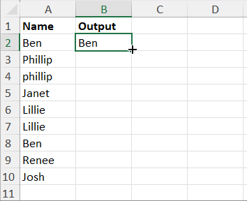
- If you have more values in column A, drag the fill handle in column B as far as you need. This is the classic method of removing case-sensitive duplicates in Excel.
How does this formula identify duplicates based on uniqueness?
The EXACT function compares two strings and returns TRUE if identical, otherwise, it returns FALSE.
For example, =EXACT("Ben", "Ben") will return TRUE, while =EXACT("Ben", "ben") will return FALSE. By using -- (double unary operator) before EXACT, we can convert TRUE to 1 and FALSE to 0.
The EXACT function can compare a name in a list and return TRUE (1) or FALSE (0) for each value. The SUMPRODUCT function then calculates the sum of these values.
In our formula in cell B1, the range is $A$1:A1, and the value to test in this range is in cell A2. In the formula in cell B2, the range is $A$1:A2, and the value to test is A3.
This means that EXACT matches the current row’s name with the names in the rows above. If it equals 0, the formula returns the name; otherwise, it returns blank.
Dynamic Array Formula for Removing Case-Sensitive Duplicates in Excel
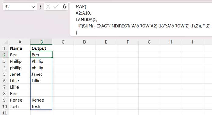
If you are using an Excel version that supports dynamic arrays and the MAP function, you can utilize the following formula in cell B2 after clearing any existing values in B2:B10:
=MAP(
   A2:A10,
   LAMBDA(Σ,
      IF(SUM(--EXACT(INDIRECT("A"&ROW(A2)-1&":A"&ROW(Σ)-1),Σ)),"",Σ)
   )
)
This dynamic array formula will remove case-sensitive duplicates in Excel in a flash.
If you’re an Excel enthusiast, you might find this formula interesting to learn. Here’s how we convert the classic formula that finds and removes case-sensitive duplicates to an Excel dynamic array formula:
Classic formula in cell B2:
=IF(SUMPRODUCT(--EXACT($A$1:A1,A2)),"", A2) // we have already seen itLet’s convert it to a Lambda function. Lambda function in cell B2:
=LAMBDA(Σ, IF(SUMPRODUCT(--EXACT($A$1:A1,Σ)),"", Σ))(A2) // we will remove this highlighted part later onWe have used the LAMBDA to define the name Σ to A2 and used the name instead of A2 in the formula expression. If you drag this formula down, you will get the exact results that the classic formula gives.
We drag the formula to iterate each element in the array. We can do that automatically using the MAP function in Excel in Microsoft 365.
In MAP, specify the array B2:B10, and use the LAMBDA function in the syntax MAP(array, lambda), where the array is A2:A10 and the lambda is the above lambda formula except for the yellow highlighted part.
=MAP(A2:A10, LAMBDA(Σ, IF(SUMPRODUCT(--EXACT($A$1:A1,Σ)),"", Σ)))Now, to increment A1 in $A$1:A1, replace $A$1:A1 with INDIRECT("A"&ROW(A2)-1&":A"&ROW(Σ)-1), and voila!
Finally, you can replace SUMPRODUCT with SUM (optional).
That is the transition from an Excel classic formula to a dynamic array formula, in the simplest possible way.
Excel Resources
- Running Count of Occurrences in Excel (Includes Dynamic Array)
- Custom Sort in Excel (Using Command and Formula)
- Flip a Table Vertically in Excel (Includes Dynamic Array Formula)
- XMATCH vs MATCH in Excel (New vs Old)
- Unpivot Excel Data Fast: Power Query & Dynamic Array Formula
- Split Text to Columns Using a Formula in Excel (Dynamic Array)
- Creating a Running Balance with Dynamic Array Formulas in Excel
- How the EXACT Function Differs in Excel and Google Sheets
- Running Total Array Formula in Excel [Formula Options]
- Address of the Last Non-Empty Cell Ignoring Blanks in a Column in Excel


