


WRAPCOLS is an array function in Google Sheets specifically for transforming a row or column into multiple columns.
Of course, we can use multiple OFSSETs, QUERY, or a VLOOKUP and SEQUENCE combo to transform values in a row or column into a two-dimensional array.
Most of us were following one of those approaches, right?
But one of the best and easiest ways is using the WRAPCOLS function.
The other one is WRAPROWS, which we learned in my recent tutorial here.
How do they differ in functionality?
WRAPCOLS returns the results in columns, whereas the WRAPROWS in rows.
Syntax and Arguments
Syntax: WRAPCOLS(range, wrap_count, [pad_with])
Arguments in the WRAPCOLS Function:
range:- The array or range to wrap. It can be in a single column or row.
wrap_count:- A number representing the maximum number of cells for each column in the output.
If wrap_count isn’t a whole number (e.g., 5.5), the function will round it down to the nearest whole number (5 here).
pad_with – It’s an optional argument in the WRAPCOLS array function to replace #N/A in blank cells with a given value.
For example, if there are ten cells in the range and the wrap_count is 6, the formula will return #N/A in the eleventh and twelfth cells.
How to Use the WRAPCOLS Function in Google Sheets
In the following example, Q1, Q2, Q3, and Q4 month-wise sales values are entered in a column under corresponding labels.
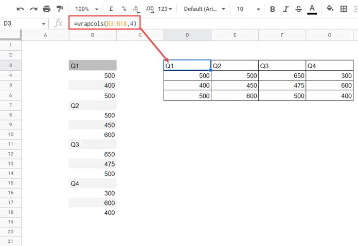
I’ve used the below WRAPCOLS formula in cell D3 to transform that data into multiple columns. So we will get each quarter’s data in different columns.
=wrapcols(B3:B18,4)In the formula the range is B3:B18 and the wrap_count is 4.
The WRAPCOLS function is one of the new functions in Google Sheets.
So, I was using the below combination formula for this purpose.
WRAPCOLS Alternative:
=ArrayFormula(vlookup(transpose(sequence(4,4,row(B3))),{row(B3:B18),B3:B18},2,0))Important:- We have used a column range in the above formula. But it can be a row also. There won’t be any changes except the range reference in the formula.
Pad_With Argument
=wrapcols(A1:A5,3)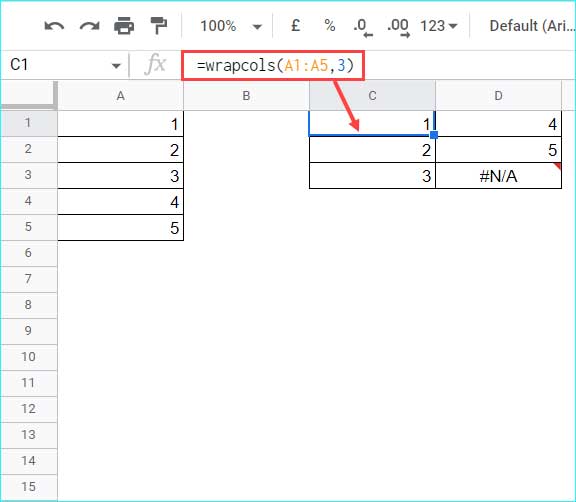
The range in the above WRAPCOLS function contains five elements.
Since the wrap_count is 3, the third cell in the second column is blank. So the formula returns #N/A!
To replace it with “no value,” use the following formula with the pad_with value.
=wrapcols(A1:A5,3,"no value")WRAPCOLS Function and Sorting a Two-Dimensional Array
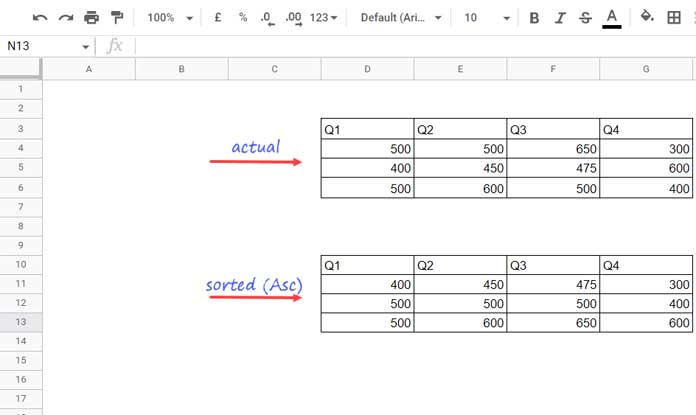
We have the sales values under Q1, Q2, Q3, and Q4 columns in D3:G6 as per screenshot # 1 above.
How do we sort the monthly sales under each column using a single piece of code?
Sorting a Two-Dimensional Array in Asc Order
Let me code the formula in a few steps that may help you understand its functioning.
We will use the WRAPCOLS function in the final step only.
Copy the field labels in D3:G3 and paste them into D10:G10.
We have a 3 x 4 (three rows and four columns) matrix leaving the header row. Use the following MAKEARRAY formula to generate a similar-size matrix.
=makearray(3,4,lambda(r,c,c+0))Flatten it.
=flatten(makearray(3,4,lambda(r,c,c+0)))Flatten the values except for the field labels.
=flatten(D4:G6)Combine the above two formulas to make a two-column array.
={flatten(makearray(3,4,lambda(r,c,c+0))),flatten(D4:G6)}The first column represents field labels, and the second column the actual values.
Sort it based on column 1 (field labels) in Asc order and column 2 (sales figures) also in Asc order.
=sort({flatten(makearray(3,4,lambda(r,c,c+0))),flatten(D4:G6)},1,1,2,1)Extract the second column using the INDEX function.
=index(sort({flatten(makearray(3,4,lambda(r,c,c+0))),flatten(D4:G6)},1,1,2,1),0,2)Then use the WRAPCOLS to wrap the above one-dimensional array into a two-dimensional array.
=wrapcols(index(sort({flatten(makearray(3,4,lambda(r,c,c+0))),flatten(D4:G6)},1,1,2,1),0,2),3)That’s the formula in cell D11.
Sorting a Two-Dimensional Array in Desc Order
Making only one change in the above formula is enough to sort the sales values in descending order.
The 1,1,2,1 parameters belong to the SORT function, and the last 1 represents the second column sort order.
Use 0 (zero) to replace it, and voila!
=wrapcols(index(sort({flatten(makearray(3,4,lambda(r,c,c+0))),flatten(D4:G6)},1,1,2,0),0,2),3)That’s all about how to use the WRAPCOLS function in Google Sheets. Thanks for the stay. Enjoy!