


You won’t learn how to use the IF Function in Google Sheets Query from my tutorial below without revealing its purpose upfront.
Firstly, let me prepare some sample data to experiment with the IF statement in Query. Afterward, I’ll explain its purpose.
Sample Data for IF Logical Formula Test in Query
On your Google Sheets, apply the formula below to cell A1 to obtain the necessary sample data for understanding the use of the IF Statement in the Query Where Clause.
=QUERY(IMPORTHTML("https://en.wikipedia.org/wiki/List_of_best-selling_fiction_authors", "Table", 1), "Select Col1, Col7")I won’t be explaining the IMPORTHTML-based formula above. If you’re unfamiliar with using this formula, please refer to my Google Sheets Function Guide and select IMPORTHTML from there.
The formula above retrieves a seven-column table from a Wikipedia page, excluding columns 2 to 6 with the QUERY function.
Here’s a partial screenshot of the imported and queried data above.

With this sample data, which lists the best-selling authors in the fiction category, you can learn how to utilize the IF function in Google Sheets Query.
The Purpose of the IF Function in Google Sheets Query
I hope you have now imported the table above into your Google Spreadsheet.
If, for any reason, you cannot import the data, you can refer to the screenshot above and prepare the data based on it. That will be sufficient.
Now, let’s delve into the purpose of the IF function in the Query formula.
Typically, the IF logical test is utilized in Query to add dynamism to the filter. To grasp this concept, start by creating a drop-down menu in cell D2.
Creating a Drop-Down for the Test:
Follow the steps below to create a data validation drop-down menu for the Query filter:
- Navigate to cell D2.
- Then, go to the menu Insert and click Drop-down. This action will insert a drop-down menu in cell D2 and open the “Data validation rules” panel on the sidebar.
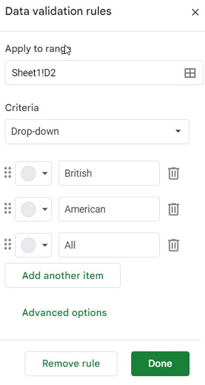
- In the rules panel, you’ll find two list items: “Option 1” and “Option 2”. Replace “Option 1” with “British” and “Option 2” with “American”.
- Click “Add another item” to enter “All”.
- Please input the text strings as displayed in the screenshot below. Click “Done”. Your drop-down menu is now ready in cell D2.
Understanding the Purpose:
Now, let’s filter the above two-column data based on the condition in cell D2.
From our sample data, please review the column headings in cells A1 and B1. You’ll notice that column 1 contains the names of the best-selling authors in the fiction category, and column 2 contains their citizenship details.
We aim to filter this data based on the author’s citizenship/nationality in column 2.
The filter criterion is already set up in cell D2 as a drop-down. The following formula can filter the data based on the condition in D2:
=QUERY(A1:B, "Select A where B='"&D2&"'",1)
If you select “British” in cell D2, the formula will return all the authors whose citizenship is British.
But what about the “All” criteria in D2? Since it’s not citizenship, there is no such string in column B.
By selecting this criterion from the drop-down menu, the objective is to list all authors irrespective of their citizenship. This is where we utilize the IF function in the Google Sheets Query.
In essence, the purpose of the IF statement in Query is to add dynamism to the filter (WHERE) clause.
How to Use the IF Logical Function in Google Sheets Query
Admittedly, the usage of single and double quotes in Query can be quite confusing, even for advanced users.
I, too, encounter difficulties at times due to the incorrect placement of quotes in Query. Therefore, it’s essential to pay close attention to their usage.
The formula that explains how to use the IF Function in the Where Clause in the Query function is:
=QUERY(A1:B, "Select A " & IF(D2="All",, "where B = '"&D2&"' "), 1)Please refer to the screenshot below.

Formula Explanation
If the value in cell D2 is “All”, the formula would function as below.
=QUERY(A1:B,"Select A ", 1)This is because we are combining the IF formula result with the query string "Select A" and IF returns null.
Enter the IF logical formula alone in any cell, i.e., =IF(D2="All",, "where B = '"&D2&"' "), and you’ll see that it returns blank.
Change the value in cell D2 to “American.” The output of the IF formula will be as follows:

In this case, the Query string in the formula would be as follows: "Select A where B = 'American'". The formula would function as follows:
=QUERY(A1:B, "Select A where B = 'American'", 1)That concludes the explanation of how to use the IF Function in Google Sheets Query.
Resources
Here are some related topics:
Hi Prashanth,
I have an issue with an IFS function working in cell C4 of the undermentioned sheet.
The function is to confirm if cells A4:A259 are less than the average in cell A260 and if cells in B4:B259 are greater than the average in B260.
And in cells C4:C259, it should display 2 if A and B are true, 1 if only one of A or B is true, or blank if neither A nor B is true.
Sample Sheet: URL removed by admin
Hi, Ron,
I’ve added a lambda solution to your Sheet. I hope that helps.
THANK YOU SO MUCH, PRASHANTH!
Just for clarification, I found (after reviewing your Purpose of WHERE 1=1 blog) that I needed to add the group by A in the first
""also to make it work — so:=QUERY(A2:C,"SELECT A, count(B) WHERE 1=1 "&IF(D2="All"," group by A"," AND B = '"&D2&"' group by A"))This is brilliant! Thank you!
Hi, Prashanth! This is really helpful – thank you.
How do you include aggregations in this formula?
If I add the “group by” before the IF statement, I can get results as long as “ALL” is selected; but if I make a selection (in this example, choose British), then I get a parse error.
example:
query(A1:C,"Select A, count(B) group by A " & IF(D2="All",, “where B = '"&D2&"' "))I know the where clause should precede the Group By, but I couldn’t get that to work at all here.
Hi, Shanda Packard,
The following formula would work.
=QUERY(A1:C,"SELECT A,count(B) WHERE 1=1 "&IF(D2="All",""," AND B = '"&D2&"' group by A"))For correctly placing the “Group By” clause, please check my Query clause order guide/tutorial.
For the rest of the formula part, please check – The Purpose of WHERE 1=1 in Google Sheets Query.
Hi, I’m looking at multiple data range sources for my Query.
Sometimes the other range would not return any result at all, which causes the Query to have an error.
=QUERY({Row_Janilla;Row_Nikita},"Select * where B = 66",0)The range
Row_Janillaon its own returns values, but the rangeRow_Nikitadoes not.I’d like for the Query to still allow to look into multiple ranges from different tabs and ignore the data range if it has no result.
Can anyone help?
Hi, Jordan,
Please check this guide – How to Include Future Sheets in Formulas in Sheets.
How do you combine Query with a pivot function and with an ifs statement? Where does it fill in the formula?
Hi, Yepz,
Could you leave the URL of a Sheet that contains an example in the comment/reply?
I’ll keep that comment away from publishing.
Thanks so much for noticing me. I’ll leave the link below. TIA
Hi, Yepz,
I could understand that you want to use multiple IF logical tests in the Query WHERE clause.
The criteria are in cells F7, F8, and F10 as drop-downs.
1. If F7= “ALL AREAS”, ignore it, else consider it.
2. If F8= “ALL CLUSTER”, ignore it, else consider it.
3. If F10= “ALL PERSONNEL”, ignore it, else consider it.
The below part does that.
"WHERE"&if(F7="ALL AREAS",," lower(E)=lower('"&F7&"') and")&if(F8="ALL CLUSTER",," lower(F)=lower('"&F8&"') and")&
if(F10="ALL PERSONNEL",," lower(C)=lower('"&F10&"') and")
I’ve modified your Query formula in cell A17 (tab: “kvp”) to incorporate the same.
Wow, you fixed it. Thank you so much! I’ve never thought to put “and” inside the if statements.
How could you apply this with multiple “Where” conditions?
Hi, Lisa Hagin,
Please consider sharing a sample of your data and the result you want (sample sheet in Edit mode). I won’t publish the comment.
Hey,
I have this.
=QUERY('Raw Data'!A1:T5000,"select A,B,C,D,E,F,G,H,I,J,K,L,M,N,O,P where M = '"&W1&"'",1)I am trying when W1 is empty, the query shows all information from the database.
Could you help me? Please.
Hi,César,
You can include the IF as below in your Query formula.
=QUERY('Raw Data'!A1:T5000,"select A,B,C,D,E,F,G,H,I,J,K,L,M,N,O,P"&if(len(W1)," where M = '"&W1&"'",),1)Hi,
I have a dataset and I am trying to use the Query function using dates in my data but unable to filter the data.
So basically I have two columns – “Date 1” and “Date 2”.
I want to filter out only those data where “Date 2” is more than one month later date than “Date 1”. Could you please help me with the Query formula?
Hi, Puja,
Let me consider more than one month is equal to Date 1 + 30.
So I am going to filter out the data if Date 2 is greater than Date 1 + 30.
For this type of filtering the better function is FILTER. Here is the formula for the range A1:B (A1:A contains Date 1 and B1:B contains Date 2).
=filter(A:B,A1:A+30 < B1:B)For exactly one month, we can use the EDATE in filter as below.
=filter(A:B,edate(A1:A,1) < B1:B)Is there a way to have two filters for the data or is this too much for google sheets? For example in clothing data color (blue, red) and type (pants, socks).
In your example, I can only make one filter.
Hi, Keaton Hulme-Jones,
You should use one more drop-down and one more IF function with the Google Sheets Query.
To test, I’m adding one more column to my sample data. For that just change the Query Importhtml formula in cell A1 as below.
=query(importhtml("https://en.wikipedia.org/wiki/List_of_best-selling_fiction_authors","Table",1),"Select Col1,Col7,Col5")So we have three columns – Author, Nationality, and Genre.
We have already one drop-down in cell D2 for the “Nationality” filter. Let’s create one more drop-down in cell E2 with the following list.
All,Romance,Adventure,FantacyLet’s see how to use multiple IF functions in Google Sheets Query.
Here is our earlier formula.
=query(A1:C,"Select A " & IF(D2="All",, "where B = '"&D2&"' "),1)Change it as;
=query({A1:C},"Select * " & IF(D2="All",, "where Col2 = '"&D2&"' "),1)(formula#1)
Let’s write one more Query. This time we will use the criterion in cell E2.
=query({A1:C},"Select Col1 " & IF(E2="All",, "where Col3 = '"&E2&"' "),1)(formula#2)
In this formula#2, replace A1:C with formula#1, and here is that final formula.
=query({query({A1:C},"Select * " & IF(D2="All",, "where Col2 = '"&D2&"' "),1)},"Select Col1 " & IF(E2="All",, "where Col3 = '"&E2&"' "),1)Hi,
I need the formula to get the result as per the below table. Struggling to get the result of the last column.
The formula I have used to get the first 6 columns is;
{query(SALES!A2:Y ,"Select C, D, G, P, Sum(T), datediff(now(), todate(P)) WHERE O ='"&(A1)&"' GROUP BY C, D, G, P Label Sum(T) 'PENDING AMOUNT', datediff(now(), todate(P)) 'OVER DAYS' " ,1)}INV.DATE | INVOICE NUMBER | CUSTOMER NAME | Due Date | PENDING AMOUNT | OVER DAYS | Status
Hi, Narahari GL,
I don’t know the type of values in columns C, D, G, and P. You have not mentioned that. So if you share a mockup sheet, I would be able to assist you.
I have been looking for a way to do dynamic query criteria for a long time. Thank you so much for your help!