There is one main advantage of the use of COLUMNS function in Vlookup in Google Sheets. It brings some dynamism to your Vlookup formula.

You can replace the “index” argument in Vlookup function with the COLUMNS function. One more thing!

I just don’t want to mislead you with the title. Because if your index argument in the Vlookup formula is in an array form, instead of the function Columns, you should use Column.

Please don’t get scared by the names Vlookup Array. I’ve included simple examples for you to understand this in this Google Sheets tutorial.

In concise this tutorial about replacing Index with Columns/Column functions in Vlookup.

Syntax:

VLOOKUP(search_key, range, index, [is_sorted])

First, we can go to one normal Vlookup formula. If you replace “index” argument with the function COLUMNS, you can gain some control over the formula.

Example:

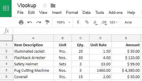
Here is a normal Vlookup Formula.

Sheets Vlookup without Columns Function

Formula 1:

=VLOOKUP("Flashback Arrester",A2:E6,5,FALSE)

This formula returns the result $120 from the Cell E3. How?

The formula above search down the first column in the range A2:E6 for the key “Flashback Arrester” and returns the corresponding value from column 5.

This column number 5 is the ‘index’ number in the above formula. Now see the use of COLUMNS function in Vlookup in Google Sheets which replaces the “index” Number.

Vlookup with Columns Function in Google Sheets

Formula 2:

=VLOOKUP("Flashback Arrester",A2:E6,COLUMNS(A2:E6),FALSE)

This Vlookup formula is also returning the same result. Here instead of index no. 5, I’ve used COLUMNS function as below which returns 5.

=COLUMNS(A2:E6)

Since there are only 5 columns in the range A2:E6 (Column A, B, C, D, and E), the Columns formula returns the number 5 as the result which is being used as the index number in Vlookup. So both the above formulas 1 and 2 return the same result from column 5.

Now let me explain to you the advantages of using COLUMNS function in Vlookup. Then we can see the COLUMN function and its array use.

Advantages of the Use of COLUMNS Function in Vlookup in Google Sheets

In one word, the Columns function bring some dynamism to the Vlookup formulas in Google Sheets.

Dynamic Vlookup Index Column

If you use Columns function in Vlookup, inserting new columns in your table has no effect on your Vlookup formula result.

Here I’ve inserted a new column in our above sample data. It’s between D and E. Let’s take a look at what happens to our two Vlookup formulas above.

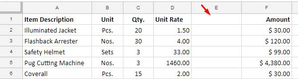
Formula 1:

=VLOOKUP("Flashback Arrester",A2:F6,5,FALSE)

This formula has no changes except the range changed from A2:E6 to A2:F6. Since the index number is still 5, the formula returns blank as there are no values in column 5 to return.

Actually, after inserting a new column, our earlier fifth column is now sixth and index number should be 6.

Formula 2:

=VLOOKUP("Flashback Arrester",A2:F6,COLUMNS(A2:F6),FALSE)

Compared to formula 1, in addition to the changes in the range, the reference in the Columns formula has also got changed.

So the Columns formula would now return the number 6, not 5 because the number of columns is now 6.

So it correctly returns the value $120. That’s what I’ve said, Columns function brings some dynamism to Vlookup in Google Sheets.

If you use the Columns function in Vlookup, no need for you to edit the formula each time when you add or delete columns in the range. Otherwise, you should have left with the option Index Match.

Is there any other use of COLUMNS function in Vlookup in Google Sheets?

Nope! There is one more advantage if you use COLUMN here, not COLUMNS.

Replacing Index in Vlookup with Column Function

In an earlier tutorial, I’ve explained to you how to use multiple index arguments in Vlookup as an Array in Google Sheets.

If you haven’t seen that tutorial, you can follow the below link. Anyway, I’m again going to give you some insight about that use below.

Must Check: Multiple Values Using Vlookup in Google Sheets is Possible

Example:

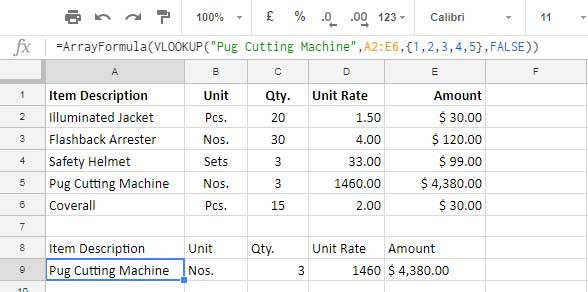
See the formula in Cell A9. There is only one search value, i.e. “Pug Cutting Machine”. But there are multiple index numbers (column output) in the result. The below is the formula used in A9.

Formula 3:

=ArrayFormula(VLOOKUP("Pug Cutting Machine",A2:E6,{1,2,3,4,5},FALSE))

It’s a Vlookup ArrayFormula as the formula returns multiple column values as a result. You can refer to the above screenshot and see row # 9 there.

This’s possible because of the use of “index” as an array, like {1,2,3,4,5} in Vlookup. Now I’m replacing these index numbers in the array with COLUMN function as below.

Formula 4:

=ArrayFormula(VLOOKUP("Pug Cutting Machine",A2:E6,column(A9:E9),FALSE))

You May Also Like: Case Sensitive Reverse Vlookup Using Index Match in Google Sheets

Why have I used COLUMN function instead of COLUMNS here? To understand this just enter the below formula in your sheet.

=arrayformula(column(A9:E9))

You can see it returns the number 1, 2, 3, 4, and 5 as an array.

These are the use of COLUMNS function in Vlookup in Google Sheets (also COLUMN).