How do we remove duplicate rows (records) but keep the rows with the max value? In Google Sheets, we can use a simple formula for this.

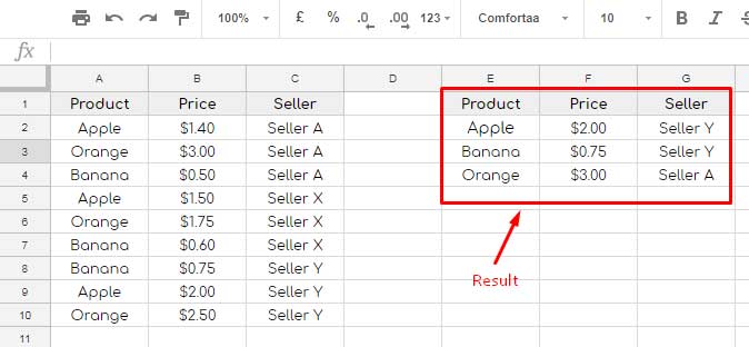
I have a table in Google Sheets, which is the price list of a few fruit items. 

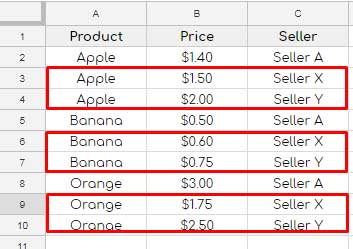
In that table, as you can see, the items are repeated multiple times but with different prices.

How can I keep only the rows that contain the highest prices?

In other words, In Google Sheets, I want to remove duplicate rows and keep the rows with the Max value in One column.

Here find the duplicates in column A, but remove them based on their price in column B.

You can see the result in the image above.

Without using any Script, you can remove duplicate rows and keep the rows with the Max value in Google Sheets.

I can proudly say this tutorial features one of the best pieces of formula you have ever used in Google Sheets for duplicate row removal!

I’ve seen people using complex formulas, such as a helper column with VLOOKUP, and a complex QUERY to get the result above.

Excel users depend mainly on Add-ons or VBA to do this. 

Unfortunately, this formula may not work in Excel as the function I use to code doesn’t exist in Excel at the time of writing this post.

Formula to Remove Duplicate Rows and Keep the Rows With Max Value

Formula:

=sortn(sort(A2:C,1,1,2,0),9^9,2,1,1)

This formula is for our data shown in the screenshot above.

You may be unable to use this formula to remove duplicate rows and keep the rows with max value in your Sheet.

Your data range may be different and has more columns.

So better, you may learn to create this formula on your own. So carefully go through my formula explanation part.

Formula Explanation

How to create a formula for duplicate row removal in google sheets based on the max value in one column?

Before starting my formula explanation section, let me share one secret about learning complex formulas.

1. Create the Sample Data (here it is the price list) as it’s in your sheet.
2. Apply the formula and check whether the result is OK.
3. Now you should split or peel the formula into several pieces depending on the number of functions used in the master formula.

Let me go straightaway to the third step.

Pealing the Master Formula

Our master formula is a single SORTN formula.

But there is one inner formula used with it as the Sortn argument (range), which is none other than the SORT.

=sort(A2:C,1,1,2,0)

This Sort formula sorts the range A2:C based on column 1 (products) in ascending order and then by column 2 (price) in descending order.

So you will get a range with the max price of products on the top of their group.

Now you are required to extract the first row from each group which is equal to removing duplicate rows and keeping the max value rows.

Final Formula

There are two built-in functions in Google Sheets to remove duplicate rows: UNIQUE and Sortn.

I’ve used the latter function.

Do you know why I haven’t used the Unique function for removing duplicates and keeping the max value (price) row?

The reason, it (Unique) is capable of removing duplicates by matching values in the total row or column.

In Sortn, the marked rows are duplicates if you choose the sort_column as 1. I’ll explain to you what is sort_column.

Syntax: SORTN(range, [n], [display_ties_mode], [sort_column], [is_ascending], [sort_column2, …], [is_ascending2, …])

range: sort(A2:C,1,1,2,0)

n: The total number of rows you want in the output. We can use an arbitrarily large number like (9^9).

sort_column: The column that determines the duplicates. Here it is the first column, so # 1.

display_ties_mode: This should be 2 to remove duplicates.

is_ascending: The output is sorted in ascending or descending order. You can put 1.

This way, you can remove duplicate rows and keep the rows with the max value in Google Sheets.