Most of the Text functions in Google Sheets are easy to use except the RE2 Regular Expression Functions like REGEXEXTRACT. In this post, I am explaining you the use of MID, SEARCH functions in Google Sheets. Both are very easy to learn.
Usage of MID, SEARCH Functions in Google Sheets
Using MID Function is a child’s play. I can give you a very clear picture of this Google Sheet Text function with few examples.
I’m going straight away to the tutorial. First, let’s me explain to you how to Use MID Function in Google Sheets.
How to Use MID Function in Google Sheets
Syntax:
MID(string, starting_at, extract_length)
The purpose of MID function is to return a certain portion or segment of a string. You can return a segment of a string from start to end.
=mid("info inspired",1,3)
Result = “inf”
In the above MID formula “info inspired” is the string, 1 is the starting_at and 3 is the extract_length.
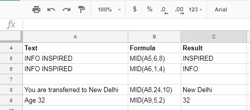
The below example is enough to understand the usage of Google Sheets MID formula.

Now it’s time to jump to the next Function. Why? See the above example at row # 8 where you can see a long text and we extracted the last portion, i.e., “New Delhi”.
Here you can see that it’s time taking to find the starting_at as you want to count each character up to New Delhi. But here we can use Google Sheets SEARCH function to find the starting_at position.
Before going to that one more thing! You can use the above MID function to split numbers into digits. Below is that advanced tutorial.
You May Like: Split Number to Digits in Google Sheets
How to Use SEARCH Function in Google Sheets
Google Sheets SEARCH function returns the position at which a string is first found within the text.
Syntax:
SEARCH(search_for, text_to_search, [starting_at])
Example:
=SEARCH("New Delhi","You are transferred to New Delhi")
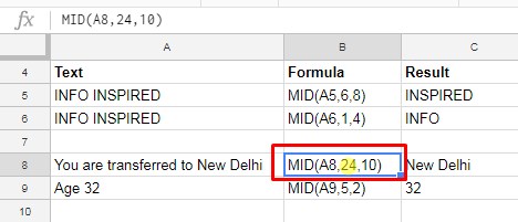
Here in this example, we search_for the word “New Delhi” within the sentence or text_to_search. So it returns 24.
This number we have used in the above MID function to extract the string “New Delhi”

When you have repeated words in your sentence, you can use the SEARCH function as below.
See the below sentence.
Note: The SEARCH function is not case sensitive.
“Moonar Tourist Destination, the best tourist destination”
Here we want to find is the position of the string “Tourist”, but the second occurrence. How to find the second occurrence of a text string using the SEARCH function?
=search("tourist","Moonar Tourist Destination, the best tourist destination")
This formula will obviously return the first position of the string tourist that is 8. So use the formula as below.
=search("tourist","Moonar Tourist Destination, the best tourist destination",9)
See the last part of this formula where I’ve added # 9. That means, as per this example, putting a number above 8 will return the second occurrence of the same word.
Tricky Ways to Extract String or Text or Word from a Sentence
See the below sentence. I want to extract the word “Kochin” form it.
“Check your mail that confirming your transfer to Kochin”
You can use four different formulas to do it. I suppose the above sentence is in Cell A19.
Formula 1 using MID function.
=MID(A19,50,7)
When you know the first part of the sentence, you can use this MID formula.
Formula 2 using MID and LEN Function Combination.
=MID(A19,LEN("Check your mail that confirming your transfer to "),7)
This is same as above. Here also you should know the first part of the sentence. But here instead of manually counting the characters, you can use LEN function inside MID.
Formula 3 using MID and SEARCH Function Combination.
=MID(A19,SEARCH("KOCHIN",A19),7)
This is different. This formula you can use when you know the text to extract but you are unsure about the first part of the sentence.
You can simplify this formula by using the Regexextract function as below.
Formula 4 using Regexextract Function
=REGEXEXTRACT(A19, "Kochin")
When you want to extract any specific test from a sentence of string, the best formula is this Regexextract.
That’s all. Hope you understand the use of MID, SEARCH Functions in Google Sheets. Enjoy!


Brilliant Prashanth. I did see the corrections in your linked tutorial and noted the missing SUM. thank you!
Dear Prashanth. Am I correct that the following code is equivalent? It seems
=if(IFERROR(search("water",A3)>0,0) OR IFERROR(search("air",A3)>0,0),"Environment","Not Environment")Equivalent to:
=if( ArrayFormula( iferror( search({"water";"air";"soil";"sky";"earth"},
A3)))>0, "Environment","Not Environment")
In this way, I can easily include more words separated by semicolons…
Hi, Jason,
The second formula is missing the SUM after the IF. It was not your mistake. In my linked tutorial (shared via my previous reply), in the first example, I forgot to include that. Corrected there and also updated your example sheet.
Dear Prashanth, I am trying to combine your powerful tutorials on IF and SEARCH.
If I have text in column O this searches the text and determines whether the word similar to water is present (water, waterfall, waterman)… and outputs Environment (if this is true)
=if(IFERROR(search("water",O3)>0,0),"Environment","Not Environment")but I want to search whether there is the word “water” or “air” in column O like this:
=if(IFERROR(search("water",O3)>0,0) OR IFERROR(search("air",O3)>0,0),"Environment","Not Environment")Hi, Jason,
Using the SEARCH function;
=if(iferror(search("water",O3))+iferror(search("air",O3))>0,"Environment","Not Environment")The above formula won’t be practical if you have to test more words in a cell. In the above example, there are only two words.
If you use REGEXMATCH, you can easily include more words separated by the Pipe as below.
=if(REGEXMATCH(O3,"water|air"),"Environment","Not Environment")If there is one more word and that is “tree”, you can include it as “water|air|tree”.
VERY CLEVER, Prashanth (SO elegant and practical…) thank you! darn… but it seems the SEARCH function can pick up “waterpick”, “waterfall”, & “underwater”… while REGEXMATCH cannot.
On a related note, can one OUTPUT whether EITHER/BOTH water or air words are present as follows?
=if(IFERROR(search("water",O3)>0,0),"water","no water") +IFERROR(search("air",O3))>0,0,"air","no air")and ideally, output “air and water” if both are present???
Hi, Jason,
The first issue with Regex you can solve by using either of the functions Lower or Upper with O3 as below.
LOWER:-
=if(REGEXMATCH(lower(O3),"water|air"),"Environment","Not Environment")UPPER:-
=if(REGEXMATCH(upper(O3),"WATER|AIR"),"Environment","Not Environment")Regarding your new requirement, try this one.
=if(and(isnumber(SEARCH("water",O3))=TRUE,isnumber(SEARCH("air",O3))=FALSE),
"water",if(and(isnumber(SEARCH("water",O3))=FALSE,
isnumber(SEARCH("air",O3))=TRUE),
"air",if(and(isnumber(SEARCH("water",O3))=TRUE,
isnumber(SEARCH("air",O3))=TRUE),
"air and water","Custom Message")))
To learn more, you may please go through this tutorial.
Logical AND, OR Use in SEARCH Function in Google Sheets.