VLOOKUP Last or Recent Record in Each Group

The easiest way to use VLOOKUP to find the last record or most recent entry in each group in Google Sheets is by flipping the data order. You don’t need to physically rearrange your data—this can be done within the VLOOKUP formula itself.

Formula to VLOOKUP Last Record in Each Group

=ArrayFormula(VLOOKUP(search_keys, SORT(range, ROW(col), FALSE), 2, FALSE))

Where:

search_keys refers to the unique values in the first column of the range.
range is the lookup range.
col is the first column in the range.

Where Is This Type of Lookup Useful?

Lookups for the last (or most recent) record in each group are valuable in various real-world scenarios. Businesses may use them to find the latest sale price of a product, while HR teams can retrieve an employee’s most recent salary or performance review. Educational institutions may track the latest fee payment status of students, and financial analysts can use them to identify the most recent transactions or cash advances taken by employees.

Example: VLOOKUP Last or Recent Record in Each Group in Google Sheets

You can use this sample sheet to test the formulas. Follow along with the steps below.

In the following example, column A contains fruit names, and column B contains their rates. Items are repeated, and the latest rates are at the bottom of the range.

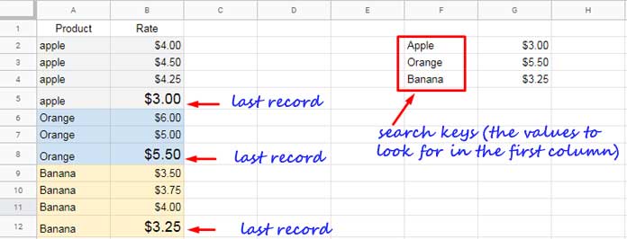
Example of using VLOOKUP to find the last record in each group

Here’s how to get the most recent rate for each unique item.

Step 1: Extract Unique Items

Enter the following formula in an empty column, such as cell F2:

=UNIQUE(A2:A)

This will return the unique items from column A.

Step 2: Use VLOOKUP to Find the Latest Rate

In cell G2, enter the following formula:

=ArrayFormula(IFNA(VLOOKUP(F2:F, SORT(A2:B, ROW(A2:A), FALSE), 2, FALSE)))

This formula will return the most recent price for each item.

Formula Explanation

F2:F – The unique items returned by the UNIQUE formula. These act as search keys in VLOOKUP.
SORT(A2:B, ROW(A2:A), FALSE) – Sorts the range by row number in descending order, effectively flipping the data.
2 – Specifies the column index (Rate column) to return the value from.
FALSE – Ensures an exact match.

The formula searches for F2:F in the flipped range and returns the first occurrence for each search key, which corresponds to the last record in the original dataset.

Why Flip the Data?

VLOOKUP always returns the first occurrence of a match. By sorting rows in descending order, we make sure the latest record appears first, allowing VLOOKUP to fetch it.

Alternative Solution Using XLOOKUP

Unlike VLOOKUP, XLOOKUP can inherently search from the bottom up, making it a more direct solution:

=ArrayFormula(XLOOKUP(F2:F, A2:A, B2:B, , 0, -1))

Formula Breakdown:

F2:F – Search keys.
A2:A – The column to search in.
B2:B – The result column.
0 – Exact match mode.
-1 – Searches from bottom to top.

Which Formula Is Better for Looking Up the Last Record in Each Group?

XLOOKUP is simpler and directly finds the last record in each group. It can look up values to the left of the result range since it allows separate search and result ranges.

However, VLOOKUP is still useful when retrieving multiple columns at once.

For example, if your data includes a third column, VLOOKUP can return multiple columns in a single formula:

=ArrayFormula(IFNA(VLOOKUP(F2:F, SORT(A2:C, ROW(A2:A), FALSE), {2, 3}, FALSE)))

With XLOOKUP, handling multiple columns requires a more complex approach using LAMBDA functions, which can be challenging for some users.

You can learn how to use XLOOKUP for multiple-column results here: XLOOKUP for Multiple Column Results in Google Sheets

FAQs

1. What if I have a date column?

If your data includes a date column, first sort by the product in ascending order and then by the date in descending order before applying VLOOKUP. This ensures that the latest entry appears first. If you prefer to use the formula provided above, sort both the product and date columns in ascending order instead.

2. Does the formula update with new data?

Yes! Since the formula uses dynamic ranges, it will automatically capture new values added to the dataset.