


With the title unstack multiple form responses in Google Sheets, I meant to say something like consolidating rows or merging rows.
Suppose, you are conducting different events and use a Google Form to collect data.
In case of multiple events and a single Form, you may want to allow multiple responses for each event.
Must Read: All that You Want to Know About Setting up of Google Docs Forms.
In this case, if you have connected your Form with Google Sheets, you may have multiple entries for the same person in your Sheets tab.
With the help of this tutorial, you can learn how to unstack multiple form responses in Google Sheets.
Here is one example for stacking multiple form responses in Google Docs Sheets.
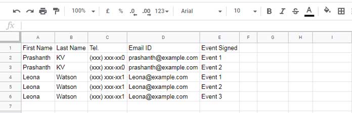
Form Response in Sheet1:
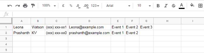
Unstacked Multiple Form Responses in Sheet2:
If this is not the type of unstacking that you are looking for, then you may check
- How to Unstack Data to Group in Google Sheets Using Formula.
- The Formula to Combine Duplicate Rows in Google Sheets.
How to Unstack Multiple Form Responses in Google Sheets
In my sample data above (Form submission), the first four columns only contain duplicate data. So what we want to do is unique these columns and transpose the fifth column that is “Event Signed”.
But unfortunately using Unique and Transpose may not going to solve this problem.
To unstack multiple form responses in Google Sheets, we can use Query string aggregation.
Instead of going into each step in Query string aggregation here, I have detailed that in a separate tutorial. See that first – How to Aggregate Strings Using Query in Google Sheets.
In that, you can see one example with two column data and in that the first column contains the duplicates. Learn that formula thoroughly.
This tutorial is an extended version of the formula presented in that tutorial. Here I have more columns to unstack.
The Formula to Unstack Multiple Form Responses in Sheets
Here is my formula for the above data range A2
You can include the Sort function within the below formula also. That detail you can find in my tutorial of which the link shared above.
=ArrayFormula(query(query({Sheet1!A2:E,if(len(Sheet1!A2:A),row(Sheet1!A2:A)-match(Sheet1!A2:A&Sheet1!B2:B,Sheet1!A2:A&Sheet1!B2:B,0),)},"Select Col1,Col2,Col3,Col4, max(Col5) where Col1 is not null group by Col1,Col2,Col3,Col4 Pivot Col6"),"Select * offset 1",0))To know how to modify this unstacking formula for a different data, you may want to compare this formula with the below example and formula.
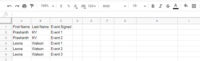
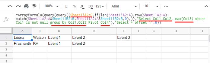
I am unstacking this three column Form response data using the below formula.
Changes in Formulas and Reason for the Change:
Changes in Data Range:
Sheet1!A2:E (5 columns) changed to Sheet1!A2:C(3 columns).
Changes in Query Select Clause:
Select Col1,Col2,Col3,Col4, changed to Select Col1,Col2, – In the first data, the first four columns contain duplicates, i.e., First N
In the second data it’s limited to two columns, i.e., First Name and Last Name.
Changes in Max Function:
max(Col5)max(Col3)
Changes in Group by Clause:
group by Col1,Col2,Col3,Col4group by Col1,Col2
Changes in Pivot Clause:
In the first example the pivot column number is 6 and in the second it’s column 4. If you check the data you can see that there are only 5 columns in the first example and 3 columns in the second.
Actually, there is one virtual column in my formula at the end of the original data. That column number comes as the pivot column in the formula.
That’s it. Follow the above two examples to learn how to unstack multiple form responses in Google Sheets.